政治学方法論 II:階層モデルとStan によるベイズ推定
矢内 勇生
2015年6月10日
準備
必要なパッケージを読み込む。必要があれば各自インストールする。 RStan のインストールについてはココ を参照。
library("reshape2")
library("dplyr")
library("ggplot2")
library("rstan")
8つの高校の並列実験 (BDA3, Section 5.5)
データ
BDA3, p.120 の表5.2 にあるデータ(平均処置効果 \(y_j\) とその標準誤差 \(\sigma_j\))を入力する。
Schools <- data.frame(y = c(28, 8, -3, 7, -1, 1, 18, 12),
                      sigma = c(15, 10, 16, 11, 9, 11, 10, 18))
J <- nrow(Schools)
ここで想定するサンプリングモデルは、 \[y_j | \theta_j \sim \mathrm{N}(\theta_j, \sigma_j^2)\] であり、\(\theta_j\) を推定するのが目的である。
8校の \(\theta\) を別々に推定する (separating)
無情報事前分布を使い、8校を別々に推定すると、各校の事後分布の95%区間は以下の図のようになる。
theta.hat.sp <- matrix(rnorm(1000 * J, mean = Schools$y, sd = Schools$sigma),
                       nrow = 1000, byrow = TRUE)
df <- data.frame(y = Schools$y,
                 median = apply(theta.hat.sp, 2, median),
                 lower = apply(theta.hat.sp, 2, function(x) quantile(x, .025)),
                 upper = apply(theta.hat.sp, 2, function(x) quantile(x, .975)))
separating <- ggplot(df, aes(x = y, y = median)) +
    geom_linerange(aes(ymin = lower, ymax = upper), col = "royalblue") +
    geom_abline(intercept = 0, slope = 1, col = "gray") +
    geom_point() +
    labs(x = expression(y[j]),
         y = expression(paste("95% posterior interval of ", theta[j])))
print(separating)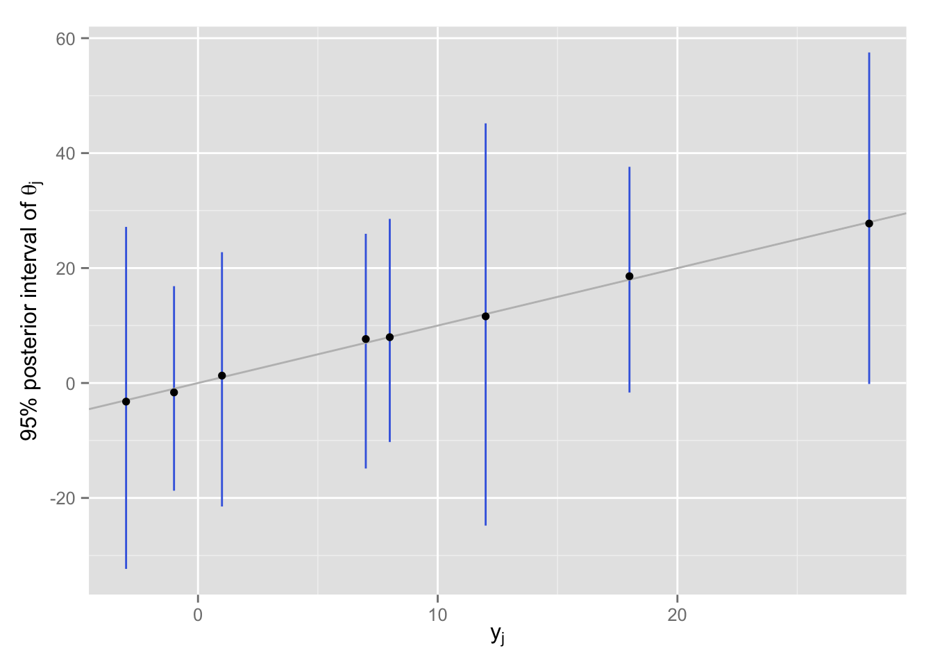
推定を別々に行っているので、点推定値(事後分布の中央値)は、\(\theta_j = y_j\) 付近にある。 推定のばらつきを見ると、すべての高校の分布が重なっており、「各校が別々の\(\theta_j\) をもつ」という前提が成り立ちそうには見えない。
8校をまとめて1つの \(\theta\) を推定する
8つの高校が共通の \(\theta\) をもつ、つまり、\(\theta_1 = \cdots = \theta_8 = \theta\) として推定する。ここでも、無情報事前分布を使う。
var.all <- 1 / sum(1 / (Schools$sigma)^2)
weight <- (1 / (Schools$sigma)^2) / var.all^(-1)
y.all <- sum(weight * Schools$y)
se.all <- sqrt(var.all)
theta.hat.pl <- rnorm(10000, mean = y.all, sd = sqrt(var.all))
quantile(theta.hat.pl, c(.025, .25, .5, .75, .975))
## 2.5% 25% 50% 75% 97.5%
## -0.4828396 4.8988249 7.6668809 10.3425117 15.6030023この分析では、平均処置効果の事後分布の中央値は約7.7である。 この推定値自体は妥当なように見える。 しかし、事後分布のばらつきを見ると、実際にA校で観察された効果である28がこの分布から出てくる可能性は著しく低いことがわかる。今回の分析でシミュレートされた10000個の値のうち、28以上の値をとった回数は、
sum(theta.hat.pl > 28)## [1] 0である。最大値は、
max(theta.hat.pl)## [1] 23.75359である。 このように、pooling モデルでは、データのばらつきをうまく説明できない。
階層モデル
階層モデルを使わない separating と pooling は極端な推定法であり、どちらもあまり 良い推定になっていないので、階層モデルを使う。
ここでは、
尤度 \[y_j | \theta_j \sim \mathrm{N}(\theta_j, \sigma_j^2)\]
事前分布 \[\theta_j | \mu, \tau \sim \mathrm{N}(\mu, \tau^2)\]
とし、
- 超事前分布は、 \[p(\mu | \tau) \propto 1\] \[p(\tau) \propto 1\] と仮定する。
同時事後分布は、 \[p(\theta, \mu, \tau | y) = p(\tau | y)p(\mu | \tau, y) p(\theta | \mu, \tau, y)\] と分解できるので、データを使い、\(\tau\)、\(\mu\)、\(\theta\) の順にシミュレート(サンプル)すればよい。
まず、\(\tau\) の周辺事後分布\(p(\tau | y)\)を求める。
mu_hat <- function(tau, y = Schools$y, sigma = Schools$sigma) {
    sum((1 / (sigma^2 + tau^2)) * y) / sum(1 / (sigma^2 + tau^2))
}
V_mu <- function(tau, sigma = Schools$sigma) {
    1 / sum(1 / (sigma^2 + tau^2))
}
post_tau <- function(tau, y = Schools$y, sigma = Schools$sigma) {
    V_mu(tau)^{1/2} *
        prod( (sigma^2 + tau^2)^{-1/2} *
             exp(-(y - mu_hat(tau))^2 / (2 * (sigma^2 + tau^2))))
}
tau <- seq(0, 30, length = 500)
post.tau.dens <- sapply(tau, post_tau)
plot(tau, post.tau.dens, type = "l", yaxt = "n",
     xlab = expression(tau), ylab = "",
     main = expression(paste("p(", tau, "|", y, ")")))
abline(v = 0, col = "gray")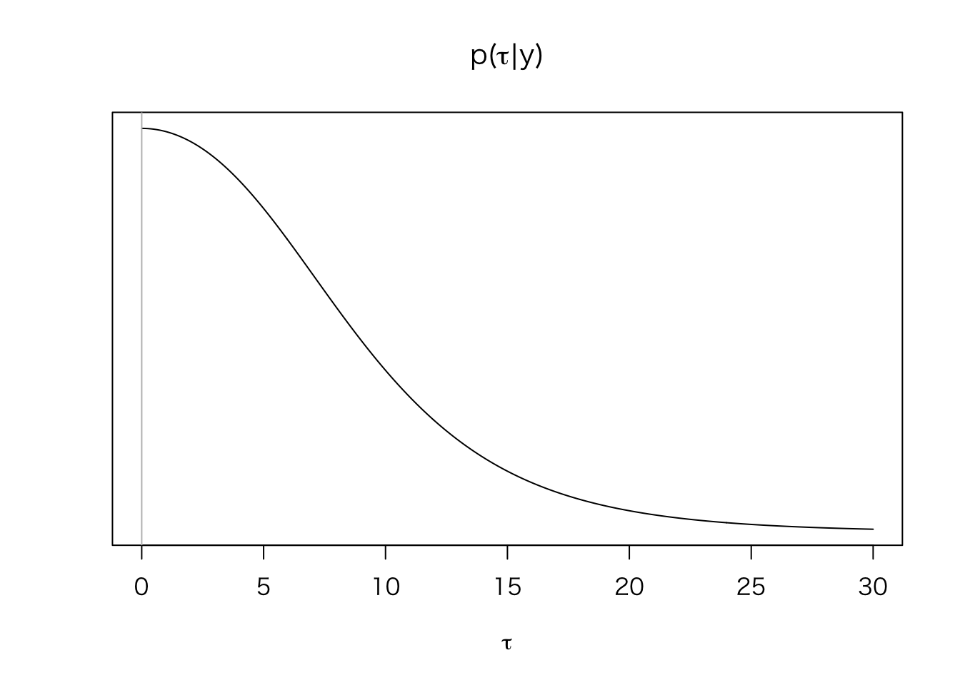
このように、\(\tau\) は0付近を取る可能性が高い(つまり、8つの学校の処置効果は異ならない可能性が高い)ことがわかる。この分布から、\(\tau\) の値をシミュレート(サンプル)する。
n.sims <- 10000
set.seed(2015-06-08)
post.tau <- sample(tau, size = n.sims, rep = TRUE,
                   prob = post.tau.dens / sum(post.tau.dens))
シミュレートされた10000個の \(\tau\) の分布をヒストグラムにしてみよう。
hist(post.tau, freq = FALSE, col = "gray",
     xlab = expression(paste(tau, "|", y)),
     main = expression(paste("10000 draws of ", tau, "|", y)))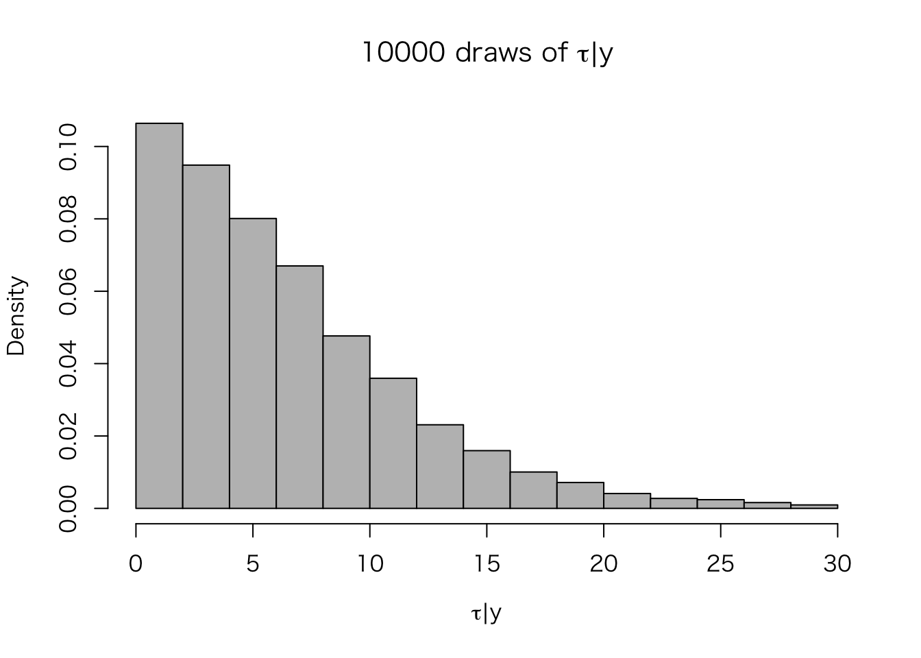
この \(\tau\) を使い、\(\mu | \tau, y \sim \mathrm{N}(\hat{\mu}, V_{\mu})\) から\(mu\) の事後分布をシミュレート(サンプル)する。
post.mu <- rnorm(n.sims, mu_hat(post.tau), sqrt(V_mu(post.tau)))
hist(post.mu, freq = FALSE, col = "gray",
     xlab = expression(paste(mu, "|", tau, ", ", y)),
     main = expression(paste("10000 draws of ", mu, "|", tau, ", ", y)))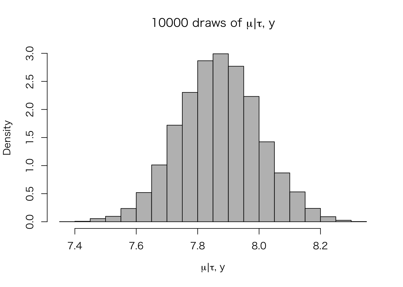
最後に、これらの値を使い、 \(\theta_j | \mu, \tau, y \sim \mathrm{N}(\hat{\theta_j}, V_j)\) から、\(\theta_j\) の事後分布をシミュレート(サンプル)する。
theta_hat <- function(mu, tau, y, sigma) {
    tau <- ifelse(tau == 0, 1e-16, tau)
    ((1 / sigma^2) * y + (1 / tau^2) * mu) / (1 / sigma^2 + 1 / tau^2)
}
V <- function(tau, sigma) {
    #tau <- ifelse(tau == 0, 1e-16, tau)
    1 / (1 / sigma^2 + 1 / tau^2)
}
post.theta <- matrix(NA, nrow = n.sims, ncol = J)
for (j in 1:J) {
    y <- Schools$y[j]
    sigma <- Schools$sigma[j]
    post.theta[, j] <- rnorm(n.sims,
                             mean = theta_hat(post.mu, post.tau, y, sigma),
                             sd = sqrt(V(post.tau, sigma)))
}各\(\theta_j\) の事後分布は、
post.theta.tbl <- t(apply(post.theta, 2,
                          function(x) quantile(x, c(.025, .25, .5, .75, .975))))
row.names(post.theta.tbl) <- paste("theta", 1:8, sep = ".")
post.theta.tbl
## 2.5% 25% 50% 75% 97.5%
## theta.1 0.6342291 7.395309 9.345745 14.139166 30.31475
## theta.2 -3.3067441 5.505440 7.890215 10.301066 18.96575
## theta.3 -9.8529234 3.698006 7.380316 9.254744 18.24775
## theta.4 -4.3433315 5.290251 7.832081 10.184733 19.60583
## theta.5 -8.2047321 2.567974 6.549038 8.333685 14.52873
## theta.6 -7.7185725 3.814626 7.229390 9.053624 16.86314
## theta.7 1.1727995 7.447684 9.268327 13.394370 25.11361
## theta.8 -5.3559398 5.785042 8.047725 11.032944 23.95859となる。 各校の事後分布の中央値は、separating の場合と異なり、極端を値をとらない(A校でも9.3)。 それと同時に、pooling の場合と異なり、データのばらつきもうまく説明できている。 A校では処置効果28が95%事後分布区間に含まれているし、C校では負の処置効果をとる確率が比較的高くなっている。 このように、階層モデルを使うと、収縮 (shrinkage) によって推定値が極端な値を取らないようにしつつ、グループ間のばらつきを捉えることが可能になる。
BDA3 の図 5.8 と同様のヒストグラムを作ってみよう。
## ggplot 用にデータフレームを作る
Post <- as.data.frame(post.theta)
names(Post) <- paste("theta", 1:8, sep = ".")
Post <- mutate(Post, largest = apply(post.theta, 1, max))
## theta.1 (A校の平均処置効果) の事後分布
hist.1 <- ggplot(Post, aes(x = theta.1, y = ..density..)) +
    geom_histogram(binwidth = 2) +
    xlim(-20, 60) +
    xlab(expression(paste("Posterior of ", theta[1])))
print(hist.1)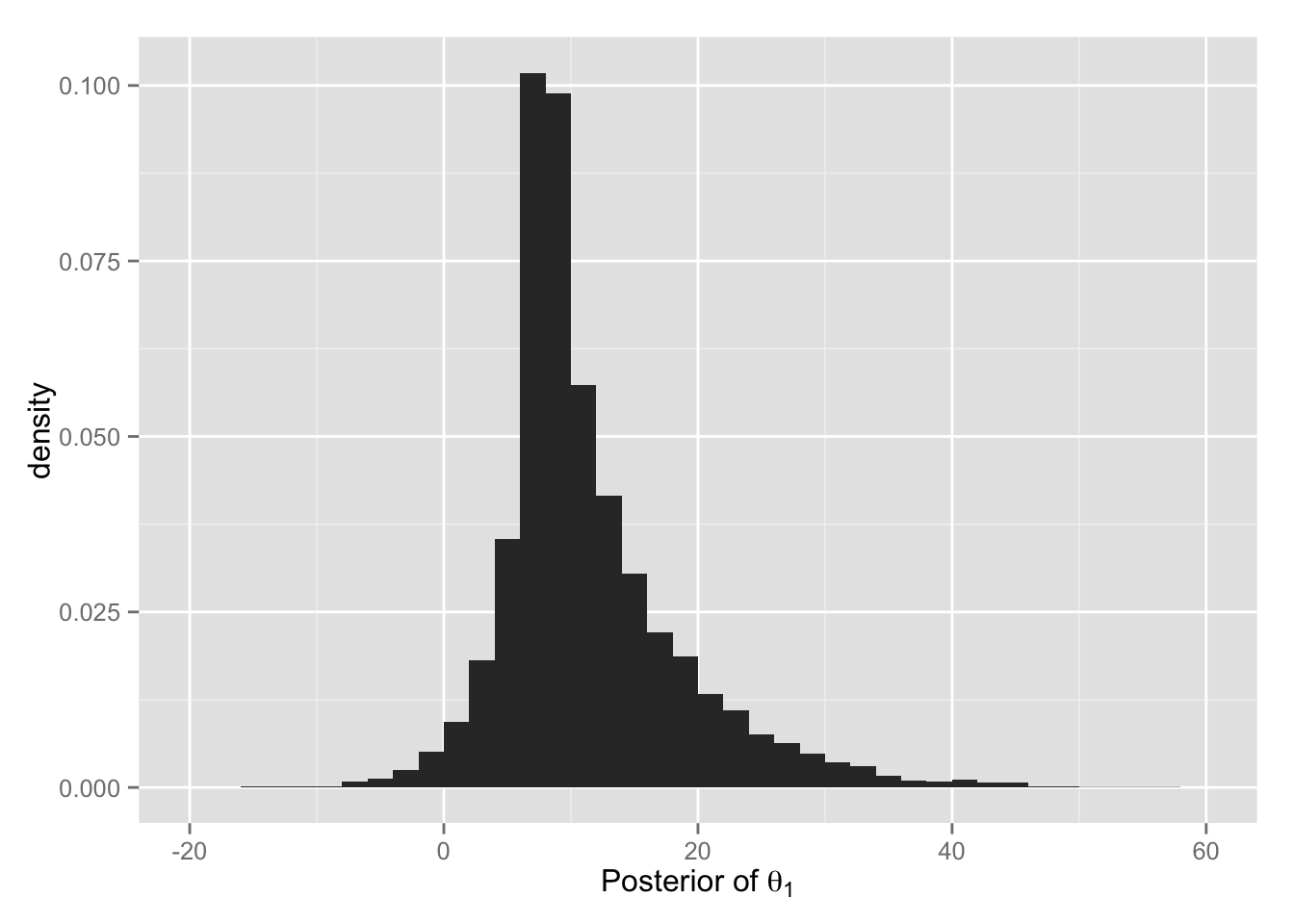
## 各シミュレーションの最大値 max(theta_j) の分布
hist.lg <- ggplot(Post, aes(x = largest, y = ..density..)) +
    geom_histogram(binwidth = 2) +
    xlim(-20, 60)
print(hist.lg)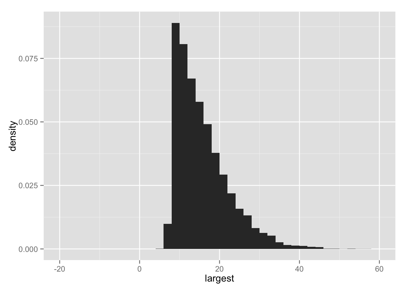
最後に、\(\theta_j\) の事後分布を示す。
Post.melt <- melt(select(Post, -largest))## No id variables; using all as measure variableshist8 <- ggplot(Post.melt, aes(x = value, y = ..density..)) +
geom_histogram(binwidth = 2) +
facet_wrap( ~ variable) +
ggtitle(expression(
paste("10000 simulation draws of posterior ", theta[j])))
hist8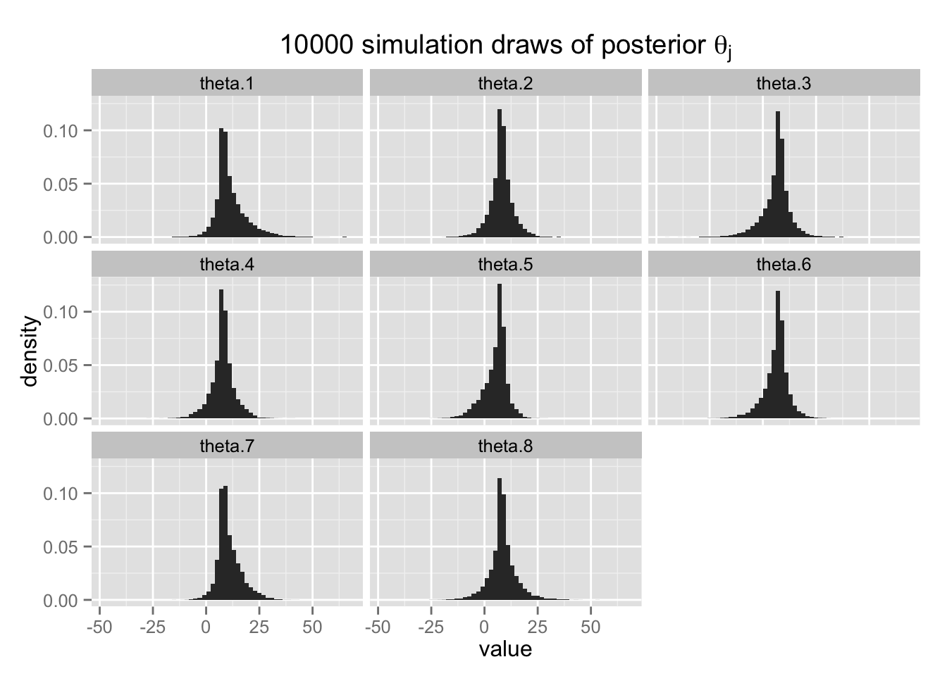
RStan による推定
ここまでの分析を Stan (RStan) で実行してみよう。
Stan を使うには、推定するモデルをstan ファイル(拡張子 .stan)に記述する。
今回は、eight-schools.stan を使う。 (ただし、本当は、eight-schools-2.stan [BDA3, p.590] のように、transformed parameters を利用したほうがよい。) このファイルの中身は、以下のとおりである。
data {
    int<lower=1> J;
    real y[J];
    real<lower=0> sigma[J];
}
parameters {
    real theta[J];
    real mu;
    real<lower=0> tau;
}
model {
    theta ~ normal(mu, tau);
    y ~ normal(theta, sigma);
}このように、data、parameters、model を指定する必要がある(場合によっては、transformed parameters も記述する)。 文法はRによく似ているが、大きな違いを(とりあえず)2つ指摘する。
第1に、各行の最後に セミコロン “;” を入力する必要がある。 これがないと、行が終了したと看做されない。 このルールは、Stan が C++ で書かれていることによる(たぶん)。
第2に、変数を宣言するときは、変数型を宣言する必要がある。 たとえば、整数型なら int を、実数型なら real を変数名の前に置く必要がある。 また、その変数が取り得る値が型以外の制限をもつなら、それも変数型同時に指定する。 たとえば、0から1の間のあたしか取らない変数(母数)pi を宣言するときは、
real<lower=0, upper=1> pi;とする。
この stan ファイルは、作業ディレクトリに保存する(もちろん、他の場所に保存し、呼び出す際に完全なパスを指定してもよい)。
Stan のモデルコードは別ファイルとして用意することを推奨するが、どうしても R スクリプトの中に含めたいときは、以下のようにモデルコード全体を文字列として変数に保存する。
eight_code <- "
data {
    int<lower=1> J;
    real y[J];
    real<lower=0> sigma[J];
}
parameters {
    real theta[J];
    real mu;
    real<lower=0> tau;
}
model {
    theta ~ normal(mu, tau);
    y ~ normal(theta, sigma);
}
"
Stan で使うデータは、リストで用意する。
Schools <- list(J = 8, y = Schools$y, sigma = Schools$sigma)これで、stan を使う準備ができた。rstan パッケージを読み込んでから、stan() で分析してみよう(chain の意味については後の授業で解説するので、今は無視してよい)。
## 必要ならパッケージを読み込む
# librar("rstan")
fit.1 <- stan(file = "eight-schools.stan", data = Schools,
              iter = 1000, chains = 4)
## 文字列で保存したモデルコードを使うときは、以下を実行
#fit.1 <- stan(model_code = eight_code, data = Schools, iter = 1000, chains = 4)
##
## TRANSLATING MODEL 'eight-schools' FROM Stan CODE TO C++ CODE NOW.
## COMPILING THE C++ CODE FOR MODEL 'eight-schools' NOW.
##
## SAMPLING FOR MODEL 'eight-schools' NOW (CHAIN 1).
##
## Iteration: 1 / 1000 [ 0%] (Warmup)
## Iteration: 100 / 1000 [ 10%] (Warmup)
## Iteration: 200 / 1000 [ 20%] (Warmup)
## Iteration: 300 / 1000 [ 30%] (Warmup)
## Iteration: 400 / 1000 [ 40%] (Warmup)
## Iteration: 500 / 1000 [ 50%] (Warmup)
## Iteration: 501 / 1000 [ 50%] (Sampling)
## Iteration: 600 / 1000 [ 60%] (Sampling)
## Iteration: 700 / 1000 [ 70%] (Sampling)
## Iteration: 800 / 1000 [ 80%] (Sampling)
## Iteration: 900 / 1000 [ 90%] (Sampling)
## Iteration: 1000 / 1000 [100%] (Sampling)
## # Elapsed Time: 0.051225 seconds (Warm-up)
## # 0.016708 seconds (Sampling)
## # 0.067933 seconds (Total)
##
##
## SAMPLING FOR MODEL 'eight-schools' NOW (CHAIN 2).
##
## Iteration: 1 / 1000 [ 0%] (Warmup)
## Iteration: 100 / 1000 [ 10%] (Warmup)
## Iteration: 200 / 1000 [ 20%] (Warmup)
## Iteration: 300 / 1000 [ 30%] (Warmup)
## Iteration: 400 / 1000 [ 40%] (Warmup)
## Iteration: 500 / 1000 [ 50%] (Warmup)
## Iteration: 501 / 1000 [ 50%] (Sampling)
## Iteration: 600 / 1000 [ 60%] (Sampling)
## Iteration: 700 / 1000 [ 70%] (Sampling)
## Iteration: 800 / 1000 [ 80%] (Sampling)
## Iteration: 900 / 1000 [ 90%] (Sampling)
## Iteration: 1000 / 1000 [100%] (Sampling)
## # Elapsed Time: 0.059376 seconds (Warm-up)
## # 0.021108 seconds (Sampling)
## # 0.080484 seconds (Total)
##
##
## SAMPLING FOR MODEL 'eight-schools' NOW (CHAIN 3).
##
## Iteration: 1 / 1000 [ 0%] (Warmup)
## Iteration: 100 / 1000 [ 10%] (Warmup)
## Iteration: 200 / 1000 [ 20%] (Warmup)
## Iteration: 300 / 1000 [ 30%] (Warmup)
## Iteration: 400 / 1000 [ 40%] (Warmup)
## Iteration: 500 / 1000 [ 50%] (Warmup)
## Iteration: 501 / 1000 [ 50%] (Sampling)
## Iteration: 600 / 1000 [ 60%] (Sampling)
## Iteration: 700 / 1000 [ 70%] (Sampling)
## Iteration: 800 / 1000 [ 80%] (Sampling)
## Iteration: 900 / 1000 [ 90%] (Sampling)
## Iteration: 1000 / 1000 [100%] (Sampling)
## # Elapsed Time: 0.056001 seconds (Warm-up)
## # 0.015078 seconds (Sampling)
## # 0.071079 seconds (Total)
##
##
## SAMPLING FOR MODEL 'eight-schools' NOW (CHAIN 4).
##
## Iteration: 1 / 1000 [ 0%] (Warmup)
## Iteration: 100 / 1000 [ 10%] (Warmup)
## Iteration: 200 / 1000 [ 20%] (Warmup)
## Iteration: 300 / 1000 [ 30%] (Warmup)
## Iteration: 400 / 1000 [ 40%] (Warmup)
## Iteration: 500 / 1000 [ 50%] (Warmup)
## Iteration: 501 / 1000 [ 50%] (Sampling)
## Iteration: 600 / 1000 [ 60%] (Sampling)
## Iteration: 700 / 1000 [ 70%] (Sampling)
## Iteration: 800 / 1000 [ 80%] (Sampling)
## Iteration: 900 / 1000 [ 90%] (Sampling)
## Iteration: 1000 / 1000 [100%] (Sampling)
## # Elapsed Time: 0.060135 seconds (Warm-up)
## # 0.026305 seconds (Sampling)
## # 0.08644 seconds (Total)推定結果の要約は print() で表示できる。
print(fit.1)## Inference for Stan model: eight-schools.
## 4 chains, each with iter=1000; warmup=500; thin=1;
## post-warmup draws per chain=500, total post-warmup draws=2000.
##
## mean se_mean sd 2.5% 25% 50% 75% 97.5% n_eff Rhat
## theta[1] 11.59 0.41 7.65 -1.84 7.16 10.06 15.22 29.83 347 1.01
## theta[2] 7.91 0.68 6.26 -4.14 4.02 7.10 12.13 20.81 86 1.06
## theta[3] 6.59 0.96 7.40 -10.30 2.80 6.92 11.35 19.78 59 1.06
## theta[4] 7.71 0.55 6.37 -5.24 4.51 7.46 12.15 19.67 134 1.03
## theta[5] 5.44 0.64 6.37 -9.01 1.69 6.68 9.42 17.20 99 1.06
## theta[6] 6.20 0.61 6.78 -8.90 2.09 7.03 10.64 18.04 125 1.04
## theta[7] 11.31 0.36 6.26 -0.84 7.31 10.85 14.67 24.35 308 1.01
## theta[8] 8.89 0.43 7.53 -5.75 4.64 8.09 13.73 25.00 313 1.03
## mu 8.23 0.58 4.90 -0.63 5.29 7.69 11.38 17.56 71 1.05
## tau 6.50 1.67 5.23 1.45 2.70 4.82 8.91 19.46 10 1.13
## lp__ -17.74 1.63 4.65 -27.11 -21.21 -17.38 -13.30 -10.82 8 1.20
##
## Samples were drawn using NUTS(diag_e) at Wed Jun 10 18:53:09 2015.
## For each parameter, n_eff is a crude measure of effective sample size,
## and Rhat is the potential scale reduction factor on split chains (at
## convergence, Rhat=1).この表のうち、右端の Rhat が推定が収束したかどうかを表す。 これについては後の授業で説明するが、Rhat が1に近づけば収束したとみなせる。 現時点では、これが1 になっていない行が複数あるので、まだ収束していないようである。
収束を目指して、さらにシミュレーションを続けよう。 Stanで1度コンパイルしたモデルをさらにシミュレートするには、引数 file (または model_code)の代わりに、fit に推定したモデルを渡す。
fit.2 <- stan(fit = fit.1, data = Schools, iter = 10000, chains = 4)##
## SAMPLING FOR MODEL 'eight-schools' NOW (CHAIN 1).
##
## Iteration: 1 / 10000 [ 0%] (Warmup)
## Iteration: 1000 / 10000 [ 10%] (Warmup)
## Iteration: 2000 / 10000 [ 20%] (Warmup)
## Iteration: 3000 / 10000 [ 30%] (Warmup)
## Iteration: 4000 / 10000 [ 40%] (Warmup)
## Iteration: 5000 / 10000 [ 50%] (Warmup)
## Iteration: 5001 / 10000 [ 50%] (Sampling)
## Iteration: 6000 / 10000 [ 60%] (Sampling)
## Iteration: 7000 / 10000 [ 70%] (Sampling)
## Iteration: 8000 / 10000 [ 80%] (Sampling)
## Iteration: 9000 / 10000 [ 90%] (Sampling)
## Iteration: 10000 / 10000 [100%] (Sampling)
## # Elapsed Time: 0.274641 seconds (Warm-up)
## # 0.210715 seconds (Sampling)
## # 0.485356 seconds (Total)
##
##
## SAMPLING FOR MODEL 'eight-schools' NOW (CHAIN 2).
##
## Iteration: 1 / 10000 [ 0%] (Warmup)
## Iteration: 1000 / 10000 [ 10%] (Warmup)
## Iteration: 2000 / 10000 [ 20%] (Warmup)
## Iteration: 3000 / 10000 [ 30%] (Warmup)
## Iteration: 4000 / 10000 [ 40%] (Warmup)
## Iteration: 5000 / 10000 [ 50%] (Warmup)
## Iteration: 5001 / 10000 [ 50%] (Sampling)
## Iteration: 6000 / 10000 [ 60%] (Sampling)
## Iteration: 7000 / 10000 [ 70%] (Sampling)
## Iteration: 8000 / 10000 [ 80%] (Sampling)
## Iteration: 9000 / 10000 [ 90%] (Sampling)
## Iteration: 10000 / 10000 [100%] (Sampling)
## # Elapsed Time: 0.237293 seconds (Warm-up)
## # 0.188304 seconds (Sampling)
## # 0.425597 seconds (Total)
##
##
## SAMPLING FOR MODEL 'eight-schools' NOW (CHAIN 3).
##
## Iteration: 1 / 10000 [ 0%] (Warmup)
## Iteration: 1000 / 10000 [ 10%] (Warmup)
## Iteration: 2000 / 10000 [ 20%] (Warmup)
## Iteration: 3000 / 10000 [ 30%] (Warmup)
## Iteration: 4000 / 10000 [ 40%] (Warmup)
## Iteration: 5000 / 10000 [ 50%] (Warmup)
## Iteration: 5001 / 10000 [ 50%] (Sampling)
## Iteration: 6000 / 10000 [ 60%] (Sampling)
## Iteration: 7000 / 10000 [ 70%] (Sampling)
## Iteration: 8000 / 10000 [ 80%] (Sampling)
## Iteration: 9000 / 10000 [ 90%] (Sampling)
## Iteration: 10000 / 10000 [100%] (Sampling)
## # Elapsed Time: 0.234052 seconds (Warm-up)
## # 0.242362 seconds (Sampling)
## # 0.476414 seconds (Total)
##
##
## SAMPLING FOR MODEL 'eight-schools' NOW (CHAIN 4).
##
## Iteration: 1 / 10000 [ 0%] (Warmup)
## Iteration: 1000 / 10000 [ 10%] (Warmup)
## Iteration: 2000 / 10000 [ 20%] (Warmup)
## Iteration: 3000 / 10000 [ 30%] (Warmup)
## Iteration: 4000 / 10000 [ 40%] (Warmup)
## Iteration: 5000 / 10000 [ 50%] (Warmup)
## Iteration: 5001 / 10000 [ 50%] (Sampling)
## Iteration: 6000 / 10000 [ 60%] (Sampling)
## Iteration: 7000 / 10000 [ 70%] (Sampling)
## Iteration: 8000 / 10000 [ 80%] (Sampling)
## Iteration: 9000 / 10000 [ 90%] (Sampling)
## Iteration: 10000 / 10000 [100%] (Sampling)
## # Elapsed Time: 0.307115 seconds (Warm-up)
## # 0.426947 seconds (Sampling)
## # 0.734062 seconds (Total)この推定結果を見てみよう。
print(fit.2)## Inference for Stan model: eight-schools.
## 4 chains, each with iter=10000; warmup=5000; thin=1;
## post-warmup draws per chain=5000, total post-warmup draws=20000.
##
## mean se_mean sd 2.5% 25% 50% 75% 97.5% n_eff Rhat
## theta[1] 11.59 0.19 8.56 -2.24 6.00 10.33 15.91 32.38 2105 1.00
## theta[2] 7.88 0.11 6.52 -5.28 3.81 7.68 12.00 21.19 3442 1.00
## theta[3] 5.85 0.13 7.91 -11.93 1.67 6.31 10.65 20.38 3825 1.00
## theta[4] 7.57 0.12 6.70 -5.99 3.35 7.39 11.80 21.00 3246 1.00
## theta[5] 4.87 0.13 6.43 -9.01 1.02 5.28 9.17 16.73 2496 1.00
## theta[6] 6.01 0.13 6.82 -8.88 2.06 6.37 10.33 18.63 2821 1.00
## theta[7] 10.83 0.15 6.86 -1.16 6.05 10.23 14.86 26.00 2056 1.00
## theta[8] 8.41 0.13 8.12 -7.44 3.75 8.12 12.85 26.26 4219 1.00
## mu 7.90 0.12 5.22 -2.06 4.55 7.73 11.13 18.26 2056 1.00
## tau 7.01 0.18 5.51 1.23 2.93 5.54 9.39 21.10 953 1.00
## lp__ -17.87 0.27 5.48 -27.84 -21.77 -18.30 -14.11 -6.79 402 1.01
##
## Samples were drawn using NUTS(diag_e) at Wed Jun 10 18:53:11 2015.
## For each parameter, n_eff is a crude measure of effective sample size,
## and Rhat is the potential scale reduction factor on split chains (at
## convergence, Rhat=1).今度は、ほとんどのRhat が1に近づいた。さらにシミュレーションの回数を増やしてみよう。
fit.3 <- stan(fit = fit.2, data = Schools, iter = 10000, chains = 4)##
## SAMPLING FOR MODEL 'eight-schools' NOW (CHAIN 1).
##
## Iteration: 1 / 10000 [ 0%] (Warmup)
## Iteration: 1000 / 10000 [ 10%] (Warmup)
## Iteration: 2000 / 10000 [ 20%] (Warmup)
## Iteration: 3000 / 10000 [ 30%] (Warmup)
## Iteration: 4000 / 10000 [ 40%] (Warmup)
## Iteration: 5000 / 10000 [ 50%] (Warmup)
## Iteration: 5001 / 10000 [ 50%] (Sampling)
## Iteration: 6000 / 10000 [ 60%] (Sampling)
## Iteration: 7000 / 10000 [ 70%] (Sampling)
## Iteration: 8000 / 10000 [ 80%] (Sampling)
## Iteration: 9000 / 10000 [ 90%] (Sampling)
## Iteration: 10000 / 10000 [100%] (Sampling)
## # Elapsed Time: 0.235248 seconds (Warm-up)
## # 0.201005 seconds (Sampling)
## # 0.436253 seconds (Total)
##
##
## SAMPLING FOR MODEL 'eight-schools' NOW (CHAIN 2).
##
## Iteration: 1 / 10000 [ 0%] (Warmup)
## Iteration: 1000 / 10000 [ 10%] (Warmup)
## Iteration: 2000 / 10000 [ 20%] (Warmup)
## Iteration: 3000 / 10000 [ 30%] (Warmup)
## Iteration: 4000 / 10000 [ 40%] (Warmup)
## Iteration: 5000 / 10000 [ 50%] (Warmup)
## Iteration: 5001 / 10000 [ 50%] (Sampling)
## Iteration: 6000 / 10000 [ 60%] (Sampling)
## Iteration: 7000 / 10000 [ 70%] (Sampling)
## Iteration: 8000 / 10000 [ 80%] (Sampling)
## Iteration: 9000 / 10000 [ 90%] (Sampling)
## Iteration: 10000 / 10000 [100%] (Sampling)
## # Elapsed Time: 0.245158 seconds (Warm-up)
## # 0.19636 seconds (Sampling)
## # 0.441518 seconds (Total)
##
##
## SAMPLING FOR MODEL 'eight-schools' NOW (CHAIN 3).
##
## Iteration: 1 / 10000 [ 0%] (Warmup)
## Iteration: 1000 / 10000 [ 10%] (Warmup)
## Iteration: 2000 / 10000 [ 20%] (Warmup)
## Iteration: 3000 / 10000 [ 30%] (Warmup)
## Iteration: 4000 / 10000 [ 40%] (Warmup)
## Iteration: 5000 / 10000 [ 50%] (Warmup)
## Iteration: 5001 / 10000 [ 50%] (Sampling)
## Iteration: 6000 / 10000 [ 60%] (Sampling)
## Iteration: 7000 / 10000 [ 70%] (Sampling)
## Iteration: 8000 / 10000 [ 80%] (Sampling)
## Iteration: 9000 / 10000 [ 90%] (Sampling)
## Iteration: 10000 / 10000 [100%] (Sampling)
## # Elapsed Time: 0.31597 seconds (Warm-up)
## # 0.289654 seconds (Sampling)
## # 0.605624 seconds (Total)
##
##
## SAMPLING FOR MODEL 'eight-schools' NOW (CHAIN 4).
##
## Iteration: 1 / 10000 [ 0%] (Warmup)
## Iteration: 1000 / 10000 [ 10%] (Warmup)
## Iteration: 2000 / 10000 [ 20%] (Warmup)
## Iteration: 3000 / 10000 [ 30%] (Warmup)
## Iteration: 4000 / 10000 [ 40%] (Warmup)
## Iteration: 5000 / 10000 [ 50%] (Warmup)
## Iteration: 5001 / 10000 [ 50%] (Sampling)
## Iteration: 6000 / 10000 [ 60%] (Sampling)
## Iteration: 7000 / 10000 [ 70%] (Sampling)
## Iteration: 8000 / 10000 [ 80%] (Sampling)
## Iteration: 9000 / 10000 [ 90%] (Sampling)
## Iteration: 10000 / 10000 [100%] (Sampling)
## # Elapsed Time: 0.257852 seconds (Warm-up)
## # 0.334305 seconds (Sampling)
## # 0.592157 seconds (Total)print(fit.3)## Inference for Stan model: eight-schools.
## 4 chains, each with iter=10000; warmup=5000; thin=1;
## post-warmup draws per chain=5000, total post-warmup draws=20000.
##
## mean se_mean sd 2.5% 25% 50% 75% 97.5% n_eff Rhat
## theta[1] 11.66 0.20 8.70 -2.20 5.88 10.21 16.19 32.57 1852 1.00
## theta[2] 7.79 0.10 6.31 -4.78 3.85 7.77 11.71 20.65 4281 1.00
## theta[3] 5.74 0.12 8.05 -12.21 1.60 6.35 10.54 20.68 4424 1.00
## theta[4] 7.49 0.10 6.61 -5.78 3.44 7.42 11.52 20.78 4052 1.00
## theta[5] 4.73 0.12 6.45 -9.62 1.05 5.09 8.97 16.55 2995 1.00
## theta[6] 5.83 0.11 6.86 -9.13 1.91 6.09 10.17 18.74 4082 1.00
## theta[7] 10.87 0.16 7.03 -1.21 6.05 10.14 15.01 26.75 1942 1.00
## theta[8] 8.39 0.13 8.25 -8.01 3.79 7.88 12.93 26.35 4296 1.00
## mu 7.81 0.10 5.29 -2.12 4.46 7.64 10.95 18.61 2654 1.00
## tau 7.23 0.23 5.66 1.15 3.12 5.82 9.67 21.35 627 1.01
## lp__ -18.11 0.31 5.50 -28.09 -21.99 -18.54 -14.37 -6.46 318 1.01
##
## Samples were drawn using NUTS(diag_e) at Wed Jun 10 18:53:13 2015.
## For each parameter, n_eff is a crude measure of effective sample size,
## and Rhat is the potential scale reduction factor on split chains (at
## convergence, Rhat=1).推定結果の概要は、plot() で図示することができる。
plot(fit.3)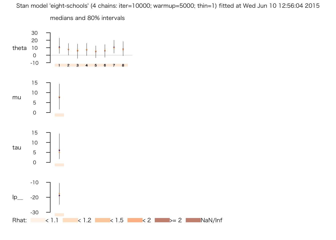
シミュレートされた値は、extract() で取り出せる。
eight.thetas <- extract(fit.3, "theta")$theta
hist(eight.thetas[, 1], freq = FALSE, col = "gray",
     xlab = expression(paste("Posterior of ", theta[1])),
     main = expression(paste("Stan's simulation draws of ", theta[1])))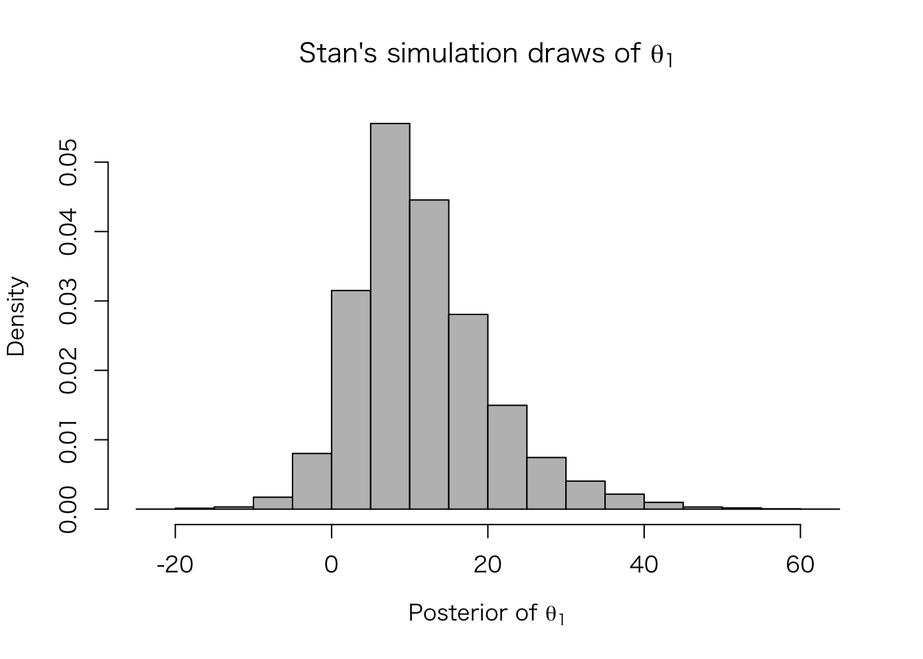
メタ分析 (BDA3, Section 5.6)
データ を読み込む。
Meta <- read.table("meta.asc", skip = 4, header = TRUE)対数オッズ比 \[y_j = \mathrm{log}\left(\frac{y_{1j}}{n_{1j} - y_{1j}}\right) - \mathrm{log}\left(\frac{y_{0j}}{n_{0j} - y_{0j}}\right)\] と、 対数オッズ比の標準誤差 \[\sigma_j = \sqrt{\frac{1}{y_{1j}} + \frac{1}{n_{1j} - y_{1j}} + \frac{1}{y_{0j}} + \frac{1}{n_{0j} - y_{0j}}}\] を計算する。 ただし、\(y_{0j}\)、\(n_{0j}\)、\(y_{1j}\)、\(n_{1j}\) はそれぞれ、研究 \(j\) における control.deaths, control.total, treated.deaths, treated.total である。
Meta <- mutate(Meta,
    y = log(treated.deaths / (treated.total - treated.deaths)) -
    log(control.deaths / (control.total - control.deaths)),
    sigma = sqrt( 1 / treated.deaths + 1 / (treated.total - treated.deaths) +
    1 / control.deaths + 1 / (control.total - control.deaths) )
    )
ここでは、各研究 \(j\) から得られた \(y_j\) が正規分布に従うと仮定する。つまり、サンプリングモデルは、 \[y_j|\theta_j \sim \mathrm{N}(\mu, \sigma_j^2)\] である。また、\(\theta_j\) の事前分布も正規分布で、 \[\theta_j | \mu, \tau \sim \mathrm{N}(\mu, \tau^2)\] であるとする。 さらに、超母数 \(\mu\)、\(\tau\) には無情報超事前分布を仮定する。 メタ分析の1つの目的は、ひとつひとつの研究だけでは推定できない、超母数 \(\mu\) を推定することである。
Stan のモデルファイルは、beta-blocker-meta.stan を使う。 中身を確認して、eight-schools.stan のモデルと比較せよ。 Rstan用にデータをリストにし、推定してみよう。
meta <- list(J = nrow(Meta), y = Meta$y, sigma = Meta$sigma)
meta.fit.1 <- stan(file = "beta-blocker-meta.stan", data = meta,
                   iter = 1000, chains = 4)
##
## TRANSLATING MODEL 'beta-blocker-meta' FROM Stan CODE TO C++ CODE NOW.
## COMPILING THE C++ CODE FOR MODEL 'beta-blocker-meta' NOW.
##
## SAMPLING FOR MODEL 'beta-blocker-meta' NOW (CHAIN 1).
##
## Iteration: 1 / 1000 [ 0%] (Warmup)
## Iteration: 100 / 1000 [ 10%] (Warmup)
## Iteration: 200 / 1000 [ 20%] (Warmup)
## Iteration: 300 / 1000 [ 30%] (Warmup)
## Iteration: 400 / 1000 [ 40%] (Warmup)
## Iteration: 500 / 1000 [ 50%] (Warmup)
## Iteration: 501 / 1000 [ 50%] (Sampling)
## Iteration: 600 / 1000 [ 60%] (Sampling)
## Iteration: 700 / 1000 [ 70%] (Sampling)
## Iteration: 800 / 1000 [ 80%] (Sampling)
## Iteration: 900 / 1000 [ 90%] (Sampling)
## Iteration: 1000 / 1000 [100%] (Sampling)
## # Elapsed Time: 0.038259 seconds (Warm-up)
## # 0.029166 seconds (Sampling)
## # 0.067425 seconds (Total)
##
##
## SAMPLING FOR MODEL 'beta-blocker-meta' NOW (CHAIN 2).
##
## Iteration: 1 / 1000 [ 0%] (Warmup)
## Iteration: 100 / 1000 [ 10%] (Warmup)
## Iteration: 200 / 1000 [ 20%] (Warmup)
## Iteration: 300 / 1000 [ 30%] (Warmup)
## Iteration: 400 / 1000 [ 40%] (Warmup)
## Iteration: 500 / 1000 [ 50%] (Warmup)
## Iteration: 501 / 1000 [ 50%] (Sampling)
## Iteration: 600 / 1000 [ 60%] (Sampling)
## Iteration: 700 / 1000 [ 70%] (Sampling)
## Iteration: 800 / 1000 [ 80%] (Sampling)
## Iteration: 900 / 1000 [ 90%] (Sampling)
## Iteration: 1000 / 1000 [100%] (Sampling)
## # Elapsed Time: 0.03597 seconds (Warm-up)
## # 0.048327 seconds (Sampling)
## # 0.084297 seconds (Total)
##
##
## SAMPLING FOR MODEL 'beta-blocker-meta' NOW (CHAIN 3).
##
## Iteration: 1 / 1000 [ 0%] (Warmup)
## Iteration: 100 / 1000 [ 10%] (Warmup)
## Iteration: 200 / 1000 [ 20%] (Warmup)
## Iteration: 300 / 1000 [ 30%] (Warmup)
## Iteration: 400 / 1000 [ 40%] (Warmup)
## Iteration: 500 / 1000 [ 50%] (Warmup)
## Iteration: 501 / 1000 [ 50%] (Sampling)
## Iteration: 600 / 1000 [ 60%] (Sampling)
## Iteration: 700 / 1000 [ 70%] (Sampling)
## Iteration: 800 / 1000 [ 80%] (Sampling)
## Iteration: 900 / 1000 [ 90%] (Sampling)
## Iteration: 1000 / 1000 [100%] (Sampling)
## # Elapsed Time: 0.043944 seconds (Warm-up)
## # 0.042643 seconds (Sampling)
## # 0.086587 seconds (Total)
##
##
## SAMPLING FOR MODEL 'beta-blocker-meta' NOW (CHAIN 4).
##
## Iteration: 1 / 1000 [ 0%] (Warmup)
## Iteration: 100 / 1000 [ 10%] (Warmup)
## Iteration: 200 / 1000 [ 20%] (Warmup)
## Iteration: 300 / 1000 [ 30%] (Warmup)
## Iteration: 400 / 1000 [ 40%] (Warmup)
## Iteration: 500 / 1000 [ 50%] (Warmup)
## Iteration: 501 / 1000 [ 50%] (Sampling)
## Iteration: 600 / 1000 [ 60%] (Sampling)
## Iteration: 700 / 1000 [ 70%] (Sampling)
## Iteration: 800 / 1000 [ 80%] (Sampling)
## Iteration: 900 / 1000 [ 90%] (Sampling)
## Iteration: 1000 / 1000 [100%] (Sampling)
## # Elapsed Time: 0.032137 seconds (Warm-up)
## # 0.063267 seconds (Sampling)
## # 0.095404 seconds (Total)エラーが出ていないことを確認し、シミュレーションの回数を増やそう。
meta.fit.2 <- stan(fit = meta.fit.1, data = meta, iter = 10000, chains = 4)##
## SAMPLING FOR MODEL 'beta-blocker-meta' NOW (CHAIN 1).
##
## Iteration: 1 / 10000 [ 0%] (Warmup)
## Iteration: 1000 / 10000 [ 10%] (Warmup)
## Iteration: 2000 / 10000 [ 20%] (Warmup)
## Iteration: 3000 / 10000 [ 30%] (Warmup)
## Iteration: 4000 / 10000 [ 40%] (Warmup)
## Iteration: 5000 / 10000 [ 50%] (Warmup)
## Iteration: 5001 / 10000 [ 50%] (Sampling)
## Iteration: 6000 / 10000 [ 60%] (Sampling)
## Iteration: 7000 / 10000 [ 70%] (Sampling)
## Iteration: 8000 / 10000 [ 80%] (Sampling)
## Iteration: 9000 / 10000 [ 90%] (Sampling)
## Iteration: 10000 / 10000 [100%] (Sampling)
## # Elapsed Time: 0.494882 seconds (Warm-up)
## # 0.503679 seconds (Sampling)
## # 0.998561 seconds (Total)
##
##
## SAMPLING FOR MODEL 'beta-blocker-meta' NOW (CHAIN 2).
##
## Iteration: 1 / 10000 [ 0%] (Warmup)
## Iteration: 1000 / 10000 [ 10%] (Warmup)
## Iteration: 2000 / 10000 [ 20%] (Warmup)
## Iteration: 3000 / 10000 [ 30%] (Warmup)
## Iteration: 4000 / 10000 [ 40%] (Warmup)
## Iteration: 5000 / 10000 [ 50%] (Warmup)
## Iteration: 5001 / 10000 [ 50%] (Sampling)
## Iteration: 6000 / 10000 [ 60%] (Sampling)
## Iteration: 7000 / 10000 [ 70%] (Sampling)
## Iteration: 8000 / 10000 [ 80%] (Sampling)
## Iteration: 9000 / 10000 [ 90%] (Sampling)
## Iteration: 10000 / 10000 [100%] (Sampling)
## # Elapsed Time: 0.29703 seconds (Warm-up)
## # 0.310046 seconds (Sampling)
## # 0.607076 seconds (Total)
##
##
## SAMPLING FOR MODEL 'beta-blocker-meta' NOW (CHAIN 3).
##
## Iteration: 1 / 10000 [ 0%] (Warmup)
## Iteration: 1000 / 10000 [ 10%] (Warmup)
## Iteration: 2000 / 10000 [ 20%] (Warmup)
## Iteration: 3000 / 10000 [ 30%] (Warmup)
## Iteration: 4000 / 10000 [ 40%] (Warmup)
## Iteration: 5000 / 10000 [ 50%] (Warmup)
## Iteration: 5001 / 10000 [ 50%] (Sampling)
## Iteration: 6000 / 10000 [ 60%] (Sampling)
## Iteration: 7000 / 10000 [ 70%] (Sampling)
## Iteration: 8000 / 10000 [ 80%] (Sampling)
## Iteration: 9000 / 10000 [ 90%] (Sampling)
## Iteration: 10000 / 10000 [100%] (Sampling)
## # Elapsed Time: 0.348975 seconds (Warm-up)
## # 0.436368 seconds (Sampling)
## # 0.785343 seconds (Total)
##
##
## SAMPLING FOR MODEL 'beta-blocker-meta' NOW (CHAIN 4).
##
## Iteration: 1 / 10000 [ 0%] (Warmup)
## Iteration: 1000 / 10000 [ 10%] (Warmup)
## Iteration: 2000 / 10000 [ 20%] (Warmup)
## Iteration: 3000 / 10000 [ 30%] (Warmup)
## Iteration: 4000 / 10000 [ 40%] (Warmup)
## Iteration: 5000 / 10000 [ 50%] (Warmup)
## Iteration: 5001 / 10000 [ 50%] (Sampling)
## Iteration: 6000 / 10000 [ 60%] (Sampling)
## Iteration: 7000 / 10000 [ 70%] (Sampling)
## Iteration: 8000 / 10000 [ 80%] (Sampling)
## Iteration: 9000 / 10000 [ 90%] (Sampling)
## Iteration: 10000 / 10000 [100%] (Sampling)
## # Elapsed Time: 0.308402 seconds (Warm-up)
## # 0.50913 seconds (Sampling)
## # 0.817532 seconds (Total)推定結果を確認してみよう。
print(meta.fit.2)## Inference for Stan model: beta-blocker-meta.
## 4 chains, each with iter=10000; warmup=5000; thin=1;
## post-warmup draws per chain=5000, total post-warmup draws=20000.
##
## mean se_mean sd 2.5% 25% 50% 75% 97.5% n_eff Rhat
## theta[1] -0.24 0.00 0.17 -0.57 -0.33 -0.24 -0.15 0.13 11382 1.00
## theta[2] -0.29 0.00 0.16 -0.65 -0.37 -0.28 -0.20 0.01 10167 1.00
## theta[3] -0.27 0.00 0.16 -0.62 -0.35 -0.27 -0.18 0.05 20000 1.00
## theta[4] -0.25 0.00 0.10 -0.44 -0.31 -0.25 -0.19 -0.05 8856 1.00
## theta[5] -0.18 0.00 0.15 -0.44 -0.28 -0.20 -0.10 0.15 4249 1.00
## theta[6] -0.27 0.00 0.17 -0.62 -0.35 -0.26 -0.18 0.07 12769 1.00
## theta[7] -0.37 0.00 0.12 -0.62 -0.44 -0.36 -0.29 -0.17 1514 1.00
## theta[8] -0.20 0.00 0.13 -0.43 -0.28 -0.21 -0.12 0.08 4641 1.00
## theta[9] -0.29 0.00 0.14 -0.58 -0.36 -0.28 -0.20 -0.03 9040 1.00
## theta[10] -0.29 0.00 0.09 -0.49 -0.35 -0.29 -0.23 -0.12 5758 1.00
## theta[11] -0.24 0.00 0.12 -0.47 -0.31 -0.24 -0.17 0.01 7757 1.00
## theta[12] -0.19 0.00 0.13 -0.43 -0.28 -0.21 -0.12 0.11 3834 1.00
## theta[13] -0.29 0.00 0.16 -0.63 -0.37 -0.28 -0.19 0.02 11675 1.00
## theta[14] -0.09 0.01 0.16 -0.34 -0.21 -0.11 0.01 0.28 1045 1.01
## theta[15] -0.26 0.00 0.14 -0.55 -0.34 -0.26 -0.18 0.03 20000 1.00
## theta[16] -0.22 0.00 0.14 -0.48 -0.31 -0.23 -0.14 0.08 20000 1.00
## theta[17] -0.19 0.00 0.15 -0.47 -0.29 -0.21 -0.11 0.16 4947 1.00
## theta[18] -0.21 0.00 0.17 -0.51 -0.30 -0.22 -0.12 0.17 6661 1.00
## theta[19] -0.22 0.00 0.17 -0.53 -0.32 -0.23 -0.13 0.17 7772 1.00
## theta[20] -0.24 0.00 0.13 -0.51 -0.32 -0.25 -0.17 0.03 20000 1.00
## theta[21] -0.33 0.00 0.14 -0.65 -0.41 -0.31 -0.23 -0.08 3442 1.00
## theta[22] -0.33 0.00 0.14 -0.66 -0.40 -0.31 -0.23 -0.07 4124 1.00
## mu -0.25 0.00 0.07 -0.37 -0.29 -0.25 -0.21 -0.11 3285 1.00
## tau 0.14 0.00 0.08 0.03 0.08 0.13 0.19 0.31 566 1.01
## lp__ 24.56 0.60 11.43 6.23 16.37 22.80 31.23 50.33 358 1.01
##
## Samples were drawn using NUTS(diag_e) at Wed Jun 10 18:53:50 2015.
## For each parameter, n_eff is a crude measure of effective sample size,
## and Rhat is the potential scale reduction factor on split chains (at
## convergence, Rhat=1).さらにシミュレーションの回数を増やしてみよう。
meta.fit.3 <- stan(fit = meta.fit.2, data = meta, iter = 20000, chains = 4)##
## SAMPLING FOR MODEL 'beta-blocker-meta' NOW (CHAIN 1).
##
## Iteration: 1 / 20000 [ 0%] (Warmup)
## Iteration: 2000 / 20000 [ 10%] (Warmup)
## Iteration: 4000 / 20000 [ 20%] (Warmup)
## Iteration: 6000 / 20000 [ 30%] (Warmup)
## Iteration: 8000 / 20000 [ 40%] (Warmup)
## Iteration: 10000 / 20000 [ 50%] (Warmup)
## Iteration: 10001 / 20000 [ 50%] (Sampling)
## Iteration: 12000 / 20000 [ 60%] (Sampling)
## Iteration: 14000 / 20000 [ 70%] (Sampling)
## Iteration: 16000 / 20000 [ 80%] (Sampling)
## Iteration: 18000 / 20000 [ 90%] (Sampling)
## Iteration: 20000 / 20000 [100%] (Sampling)
## # Elapsed Time: 0.623204 seconds (Warm-up)
## # 0.79816 seconds (Sampling)
## # 1.42136 seconds (Total)
##
##
## SAMPLING FOR MODEL 'beta-blocker-meta' NOW (CHAIN 2).
##
## Iteration: 1 / 20000 [ 0%] (Warmup)
## Iteration: 2000 / 20000 [ 10%] (Warmup)
## Iteration: 4000 / 20000 [ 20%] (Warmup)
## Iteration: 6000 / 20000 [ 30%] (Warmup)
## Iteration: 8000 / 20000 [ 40%] (Warmup)
## Iteration: 10000 / 20000 [ 50%] (Warmup)
## Iteration: 10001 / 20000 [ 50%] (Sampling)
## Iteration: 12000 / 20000 [ 60%] (Sampling)
## Iteration: 14000 / 20000 [ 70%] (Sampling)
## Iteration: 16000 / 20000 [ 80%] (Sampling)
## Iteration: 18000 / 20000 [ 90%] (Sampling)
## Iteration: 20000 / 20000 [100%] (Sampling)
## # Elapsed Time: 0.555102 seconds (Warm-up)
## # 0.677569 seconds (Sampling)
## # 1.23267 seconds (Total)
##
##
## SAMPLING FOR MODEL 'beta-blocker-meta' NOW (CHAIN 3).
##
## Iteration: 1 / 20000 [ 0%] (Warmup)
## Iteration: 2000 / 20000 [ 10%] (Warmup)
## Iteration: 4000 / 20000 [ 20%] (Warmup)
## Iteration: 6000 / 20000 [ 30%] (Warmup)
## Iteration: 8000 / 20000 [ 40%] (Warmup)
## Iteration: 10000 / 20000 [ 50%] (Warmup)
## Iteration: 10001 / 20000 [ 50%] (Sampling)
## Iteration: 12000 / 20000 [ 60%] (Sampling)
## Iteration: 14000 / 20000 [ 70%] (Sampling)
## Iteration: 16000 / 20000 [ 80%] (Sampling)
## Iteration: 18000 / 20000 [ 90%] (Sampling)
## Iteration: 20000 / 20000 [100%] (Sampling)
## # Elapsed Time: 0.661806 seconds (Warm-up)
## # 0.693748 seconds (Sampling)
## # 1.35555 seconds (Total)
##
##
## SAMPLING FOR MODEL 'beta-blocker-meta' NOW (CHAIN 4).
##
## Iteration: 1 / 20000 [ 0%] (Warmup)
## Iteration: 2000 / 20000 [ 10%] (Warmup)
## Iteration: 4000 / 20000 [ 20%] (Warmup)
## Iteration: 6000 / 20000 [ 30%] (Warmup)
## Iteration: 8000 / 20000 [ 40%] (Warmup)
## Iteration: 10000 / 20000 [ 50%] (Warmup)
## Iteration: 10001 / 20000 [ 50%] (Sampling)
## Iteration: 12000 / 20000 [ 60%] (Sampling)
## Iteration: 14000 / 20000 [ 70%] (Sampling)
## Iteration: 16000 / 20000 [ 80%] (Sampling)
## Iteration: 18000 / 20000 [ 90%] (Sampling)
## Iteration: 20000 / 20000 [100%] (Sampling)
## # Elapsed Time: 0.606764 seconds (Warm-up)
## # 0.589975 seconds (Sampling)
## # 1.19674 seconds (Total)推定結果を確認してみよう。
print(meta.fit.3)## Inference for Stan model: beta-blocker-meta.
## 4 chains, each with iter=20000; warmup=10000; thin=1;
## post-warmup draws per chain=10000, total post-warmup draws=40000.
##
## mean se_mean sd 2.5% 25% 50% 75% 97.5% n_eff Rhat
## theta[1] -0.24 0.00 0.17 -0.57 -0.33 -0.24 -0.15 0.13 19575 1.00
## theta[2] -0.29 0.00 0.16 -0.67 -0.37 -0.28 -0.20 0.01 18097 1.00
## theta[3] -0.27 0.00 0.16 -0.62 -0.35 -0.26 -0.18 0.06 22957 1.00
## theta[4] -0.25 0.00 0.10 -0.44 -0.31 -0.25 -0.19 -0.05 17044 1.00
## theta[5] -0.18 0.00 0.15 -0.44 -0.28 -0.20 -0.10 0.16 6204 1.00
## theta[6] -0.27 0.00 0.17 -0.62 -0.35 -0.26 -0.18 0.07 23548 1.00
## theta[7] -0.37 0.00 0.12 -0.62 -0.45 -0.36 -0.28 -0.18 2880 1.00
## theta[8] -0.20 0.00 0.13 -0.43 -0.28 -0.21 -0.12 0.09 5900 1.00
## theta[9] -0.29 0.00 0.14 -0.59 -0.36 -0.28 -0.20 -0.02 14223 1.00
## theta[10] -0.29 0.00 0.09 -0.48 -0.35 -0.29 -0.23 -0.12 6179 1.00
## theta[11] -0.24 0.00 0.12 -0.47 -0.31 -0.24 -0.17 0.01 15309 1.00
## theta[12] -0.19 0.00 0.13 -0.43 -0.28 -0.21 -0.11 0.11 7141 1.00
## theta[13] -0.29 0.00 0.16 -0.64 -0.37 -0.28 -0.20 0.02 20496 1.00
## theta[14] -0.08 0.00 0.16 -0.34 -0.21 -0.11 0.02 0.29 1779 1.00
## theta[15] -0.26 0.00 0.14 -0.56 -0.34 -0.26 -0.18 0.02 22722 1.00
## theta[16] -0.22 0.00 0.14 -0.48 -0.31 -0.23 -0.14 0.08 12756 1.00
## theta[17] -0.19 0.00 0.16 -0.47 -0.29 -0.21 -0.11 0.18 7497 1.00
## theta[18] -0.21 0.00 0.17 -0.51 -0.31 -0.22 -0.12 0.18 11318 1.00
## theta[19] -0.21 0.00 0.17 -0.53 -0.31 -0.23 -0.13 0.17 13962 1.00
## theta[20] -0.24 0.00 0.13 -0.51 -0.32 -0.25 -0.16 0.04 19172 1.00
## theta[21] -0.33 0.00 0.14 -0.66 -0.41 -0.31 -0.24 -0.08 6556 1.00
## theta[22] -0.33 0.00 0.15 -0.67 -0.41 -0.31 -0.23 -0.07 6988 1.00
## mu -0.25 0.00 0.07 -0.38 -0.29 -0.25 -0.21 -0.11 4881 1.00
## tau 0.14 0.00 0.08 0.03 0.08 0.13 0.19 0.32 1037 1.01
## lp__ 24.34 0.49 11.57 6.15 15.95 22.39 31.08 50.79 558 1.02
##
## Samples were drawn using NUTS(diag_e) at Wed Jun 10 18:53:56 2015.
## For each parameter, n_eff is a crude measure of effective sample size,
## and Rhat is the potential scale reduction factor on split chains (at
## convergence, Rhat=1).plot(meta.fit.3)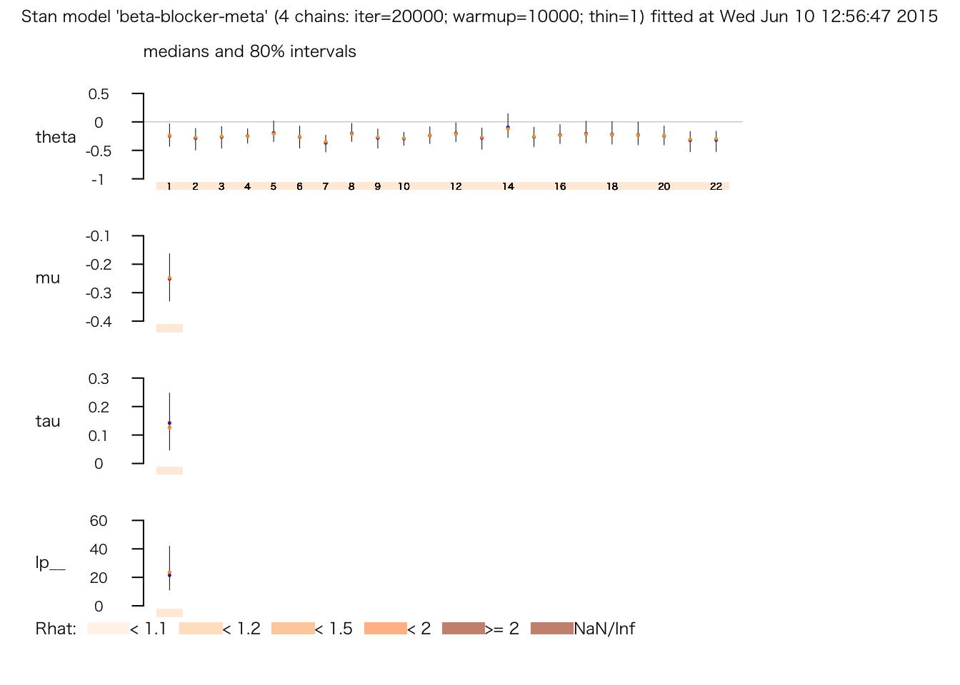
この推定における shrinkage を図示してみよう。
meta.post.theta <- extract(meta.fit.3, "theta")$theta
Meta$median <- apply(meta.post.theta, 2, median)
Meta$lower <- apply(meta.post.theta, 2, function(x) quantile(x, .025))
Meta$upper <- apply(meta.post.theta, 2, function(x) quantile(x, .975))
Meta <- mutate(Meta, total = control.total + treated.total)
## weighted mean of observed y
meta.mean <- with(Meta, sum(total * y) / sum(total))
meta.shrinkage <- ggplot(Meta, aes(x = y, y = median)) +
    geom_linerange(aes(ymin = lower, ymax = upper), color = "skyblue") +
    geom_abline(intercept = 0, slope = 1, color = "gray") +
    geom_hline(yintercept = meta.mean, color = "gray", linetype = "dashed") +
    geom_point() +
    ylim(min(Meta$y), max(Meta$y)) + coord_fixed() +
    ylab("95% posterior interval")
print(meta.shrinkage)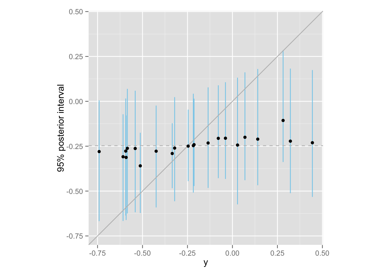
観測値の数によって、shrinkage の程度がどう変わるか確認してみよう。
Meta <- mutate(Meta, shrinkage = y - median)
meta.shrinkage.2 <- ggplot(Meta, aes(total, shrinkage)) +
    geom_point() +
    geom_hline(yintercept = 0, color = "red", linetype = "dashed") +
    xlab("total number of observations in the study")
meta.shrinkage.2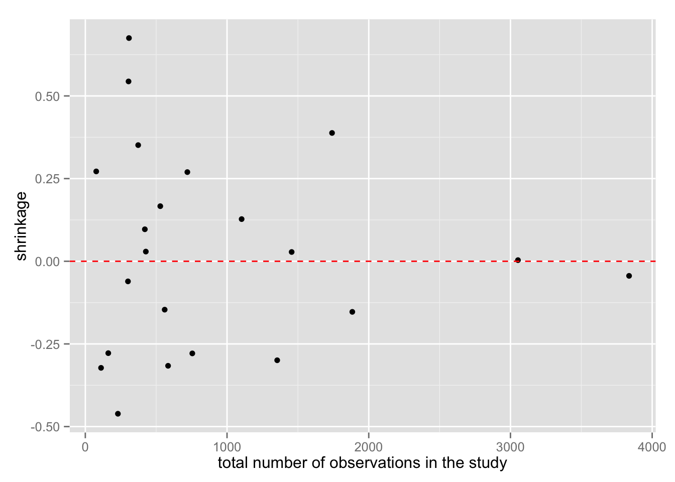
ここで、メタ分析の推定対象である、\(\mu\) の事後分布を確認してみよう。
meta.post.mu <- extract(meta.fit.3, "mu")$mu
hist(meta.post.mu, freq = FALSE, col = "gray", main = "",
     xlab = expression(paste("posterior of ", mu)))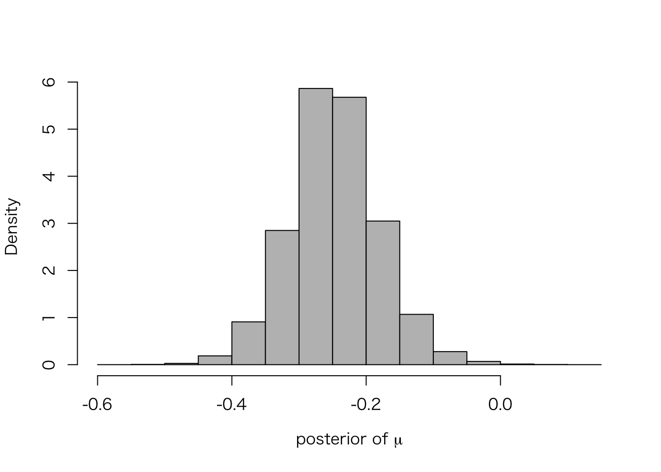
ひとつひとつの研究では \(y_j\) (separting による\(\theta_j\) の点推定値)が \(-0.74\) から\(0.44\) の範囲にばらついていたが、メタ分析すると、その超母数である \(\mu\) は非常に狭い範囲の値しかとらないことがわかる。
quantile(meta.post.mu, c(.025, .25, .5, .75, .975))## 2.5% 25% 50% 75% 97.5%
## -0.3752526 -0.2888957 -0.2485028 -0.2053270 -0.1108237このように、\(\mu|y\) の95%区間は \([-0.37, -0.11]\) である。
最後に、\(\tau\) の事後分布を確認してみよう。
meta.post.tau <- extract(meta.fit.3, "tau")$tau
hist(meta.post.tau, freq = FALSE, col = "gray", main = "",
     xlab = expression(paste("posterior of ", tau)))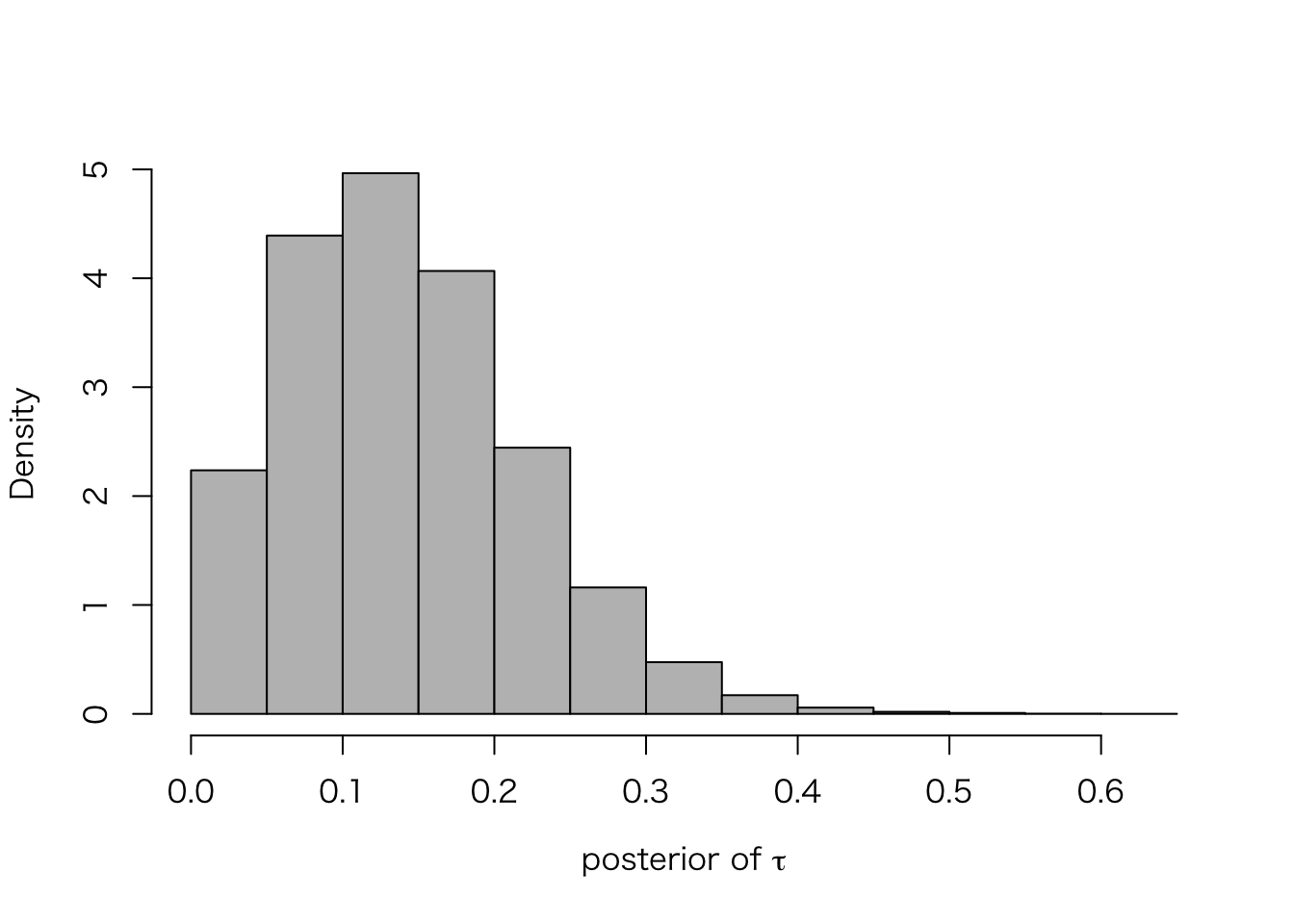
quantile(meta.post.tau, c(.025, .25, .5, .75, .975))## 2.5% 25% 50% 75% 97.5%
## 0.03139695 0.08265337 0.13411058 0.18995084 0.31847777このように、\(\tau |y\) の95%区間は \(\tau=0\) を含まない。 これは、\(\tau = 0\) を仮定する complete pooling には問題があることを示唆する。
試しに、complete pooling で分析してみよう。
y0.pool <- sum(Meta$control.deaths)
n0.pool <- sum(Meta$control.total)
y1.pool <- sum(Meta$treated.deaths)
n1.pool <- sum(Meta$treated.total)
y.pool <- log(y1.pool / (n1.pool - y1.pool)) -
          log(y0.pool / (n0.pool - y0.pool))
sigma.pool <- sqrt( 1 / y1.pool + 1 / (n1.pool - y1.pool) +
                    1 / y0.pool + 1 / (n0.pool - y0.pool) )
meta.post.mu.pool <- rnorm(10000, mean = y.pool, sd = sigma.pool)
quantile(meta.post.mu.pool, c(.025, .25, .5, .75, .975))
## 2.5% 25% 50% 75% 97.5%
## -0.3544419 -0.2903427 -0.2564926 -0.2232557 -0.1601768このように、pooling した場合あの95%事後区間は非常に狭く、データに顕われるばらつきをうまく捉えていない。
RStan の練習
先週までに推定したモデルを、RStan を使って推定し直してみよう。
生物学的検定実験
Stan で推定するために、推定モデルを .stan ファイルに記述する。 ここでは、bioassay.stan にモデルが記述されている。 このファイルの中身は、以下のとおりである。
data {
    int<lower=0> J;
    int<lower=0> y[J];
    int<lower=1> n[J];
    real x[J];
}
parameters {
    real alpha;
    real beta;
}
transformed parameters {
    real<lower=0, upper=1> theta[J];
    for (j in 1:J) {
        theta[j] <- 1 / (1 + exp(-alpha - beta * x[j]));
    }
}
model {
    y ~ binomial(n, theta);
}
データをリストとして用意する。
Bio <- list(x = c(-0.86, -0.3, -0.05, 0.73),
            n = rep(5, 4),
            y = c(0, 1, 3, 5),
            J = 4)
Stan で推定する。
bio.fit.1 <- stan(file = "bioassay.stan", data = Bio, iter = 1000, chains = 4)##
## TRANSLATING MODEL 'bioassay' FROM Stan CODE TO C++ CODE NOW.
## COMPILING THE C++ CODE FOR MODEL 'bioassay' NOW.
##
## SAMPLING FOR MODEL 'bioassay' NOW (CHAIN 1).
##
## Iteration: 1 / 1000 [ 0%] (Warmup)
## Iteration: 100 / 1000 [ 10%] (Warmup)
## Iteration: 200 / 1000 [ 20%] (Warmup)
## Iteration: 300 / 1000 [ 30%] (Warmup)
## Iteration: 400 / 1000 [ 40%] (Warmup)
## Iteration: 500 / 1000 [ 50%] (Warmup)
## Iteration: 501 / 1000 [ 50%] (Sampling)
## Iteration: 600 / 1000 [ 60%] (Sampling)
## Iteration: 700 / 1000 [ 70%] (Sampling)
## Iteration: 800 / 1000 [ 80%] (Sampling)
## Iteration: 900 / 1000 [ 90%] (Sampling)
## Iteration: 1000 / 1000 [100%] (Sampling)
## # Elapsed Time: 0.015181 seconds (Warm-up)
## # 0.013404 seconds (Sampling)
## # 0.028585 seconds (Total)
##
##
## SAMPLING FOR MODEL 'bioassay' NOW (CHAIN 2).
##
## Iteration: 1 / 1000 [ 0%] (Warmup)
## Iteration: 100 / 1000 [ 10%] (Warmup)
## Iteration: 200 / 1000 [ 20%] (Warmup)
## Iteration: 300 / 1000 [ 30%] (Warmup)
## Iteration: 400 / 1000 [ 40%] (Warmup)
## Iteration: 500 / 1000 [ 50%] (Warmup)
## Iteration: 501 / 1000 [ 50%] (Sampling)
## Iteration: 600 / 1000 [ 60%] (Sampling)
## Iteration: 700 / 1000 [ 70%] (Sampling)
## Iteration: 800 / 1000 [ 80%] (Sampling)
## Iteration: 900 / 1000 [ 90%] (Sampling)
## Iteration: 1000 / 1000 [100%] (Sampling)
## # Elapsed Time: 0.014978 seconds (Warm-up)
## # 0.010343 seconds (Sampling)
## # 0.025321 seconds (Total)
##
##
## SAMPLING FOR MODEL 'bioassay' NOW (CHAIN 3).
##
## Iteration: 1 / 1000 [ 0%] (Warmup)
## Iteration: 100 / 1000 [ 10%] (Warmup)
## Iteration: 200 / 1000 [ 20%] (Warmup)
## Iteration: 300 / 1000 [ 30%] (Warmup)
## Iteration: 400 / 1000 [ 40%] (Warmup)
## Iteration: 500 / 1000 [ 50%] (Warmup)
## Iteration: 501 / 1000 [ 50%] (Sampling)
## Iteration: 600 / 1000 [ 60%] (Sampling)
## Iteration: 700 / 1000 [ 70%] (Sampling)
## Iteration: 800 / 1000 [ 80%] (Sampling)
## Iteration: 900 / 1000 [ 90%] (Sampling)
## Iteration: 1000 / 1000 [100%] (Sampling)
## # Elapsed Time: 0.012403 seconds (Warm-up)
## # 0.007994 seconds (Sampling)
## # 0.020397 seconds (Total)
##
##
## SAMPLING FOR MODEL 'bioassay' NOW (CHAIN 4).
##
## Iteration: 1 / 1000 [ 0%] (Warmup)
## Iteration: 100 / 1000 [ 10%] (Warmup)
## Iteration: 200 / 1000 [ 20%] (Warmup)
## Iteration: 300 / 1000 [ 30%] (Warmup)
## Iteration: 400 / 1000 [ 40%] (Warmup)
## Iteration: 500 / 1000 [ 50%] (Warmup)
## Iteration: 501 / 1000 [ 50%] (Sampling)
## Iteration: 600 / 1000 [ 60%] (Sampling)
## Iteration: 700 / 1000 [ 70%] (Sampling)
## Iteration: 800 / 1000 [ 80%] (Sampling)
## Iteration: 900 / 1000 [ 90%] (Sampling)
## Iteration: 1000 / 1000 [100%] (Sampling)
## # Elapsed Time: 0.017851 seconds (Warm-up)
## # 0.011178 seconds (Sampling)
## # 0.029029 seconds (Total)シミュレーションの回数を増やす。
bio.fit.2 <- stan(fit = bio.fit.1, data = Bio, iter = 10000, chains = 4)##
## SAMPLING FOR MODEL 'bioassay' NOW (CHAIN 1).
##
## Iteration: 1 / 10000 [ 0%] (Warmup)
## Iteration: 1000 / 10000 [ 10%] (Warmup)
## Iteration: 2000 / 10000 [ 20%] (Warmup)
## Iteration: 3000 / 10000 [ 30%] (Warmup)
## Iteration: 4000 / 10000 [ 40%] (Warmup)
## Iteration: 5000 / 10000 [ 50%] (Warmup)
## Iteration: 5001 / 10000 [ 50%] (Sampling)
## Iteration: 6000 / 10000 [ 60%] (Sampling)
## Iteration: 7000 / 10000 [ 70%] (Sampling)
## Iteration: 8000 / 10000 [ 80%] (Sampling)
## Iteration: 9000 / 10000 [ 90%] (Sampling)
## Iteration: 10000 / 10000 [100%] (Sampling)
## # Elapsed Time: 0.115217 seconds (Warm-up)
## # 0.123391 seconds (Sampling)
## # 0.238608 seconds (Total)
##
##
## SAMPLING FOR MODEL 'bioassay' NOW (CHAIN 2).
##
## Iteration: 1 / 10000 [ 0%] (Warmup)
## Iteration: 1000 / 10000 [ 10%] (Warmup)
## Iteration: 2000 / 10000 [ 20%] (Warmup)
## Iteration: 3000 / 10000 [ 30%] (Warmup)
## Iteration: 4000 / 10000 [ 40%] (Warmup)
## Iteration: 5000 / 10000 [ 50%] (Warmup)
## Iteration: 5001 / 10000 [ 50%] (Sampling)
## Iteration: 6000 / 10000 [ 60%] (Sampling)
## Iteration: 7000 / 10000 [ 70%] (Sampling)
## Iteration: 8000 / 10000 [ 80%] (Sampling)
## Iteration: 9000 / 10000 [ 90%] (Sampling)
## Iteration: 10000 / 10000 [100%] (Sampling)
## # Elapsed Time: 0.118718 seconds (Warm-up)
## # 0.113659 seconds (Sampling)
## # 0.232377 seconds (Total)
##
##
## SAMPLING FOR MODEL 'bioassay' NOW (CHAIN 3).
##
## Iteration: 1 / 10000 [ 0%] (Warmup)
## Iteration: 1000 / 10000 [ 10%] (Warmup)
## Iteration: 2000 / 10000 [ 20%] (Warmup)
## Iteration: 3000 / 10000 [ 30%] (Warmup)
## Iteration: 4000 / 10000 [ 40%] (Warmup)
## Iteration: 5000 / 10000 [ 50%] (Warmup)
## Iteration: 5001 / 10000 [ 50%] (Sampling)
## Iteration: 6000 / 10000 [ 60%] (Sampling)
## Iteration: 7000 / 10000 [ 70%] (Sampling)
## Iteration: 8000 / 10000 [ 80%] (Sampling)
## Iteration: 9000 / 10000 [ 90%] (Sampling)
## Iteration: 10000 / 10000 [100%] (Sampling)
## # Elapsed Time: 0.124278 seconds (Warm-up)
## # 0.124644 seconds (Sampling)
## # 0.248922 seconds (Total)
##
##
## SAMPLING FOR MODEL 'bioassay' NOW (CHAIN 4).
##
## Iteration: 1 / 10000 [ 0%] (Warmup)
## Iteration: 1000 / 10000 [ 10%] (Warmup)
## Iteration: 2000 / 10000 [ 20%] (Warmup)
## Iteration: 3000 / 10000 [ 30%] (Warmup)
## Iteration: 4000 / 10000 [ 40%] (Warmup)
## Iteration: 5000 / 10000 [ 50%] (Warmup)
## Iteration: 5001 / 10000 [ 50%] (Sampling)
## Iteration: 6000 / 10000 [ 60%] (Sampling)
## Iteration: 7000 / 10000 [ 70%] (Sampling)
## Iteration: 8000 / 10000 [ 80%] (Sampling)
## Iteration: 9000 / 10000 [ 90%] (Sampling)
## Iteration: 10000 / 10000 [100%] (Sampling)
## # Elapsed Time: 0.097433 seconds (Warm-up)
## # 0.141082 seconds (Sampling)
## # 0.238515 seconds (Total)print(bio.fit.2)## Inference for Stan model: bioassay.
## 4 chains, each with iter=10000; warmup=5000; thin=1;
## post-warmup draws per chain=5000, total post-warmup draws=20000.
##
## mean se_mean sd 2.5% 25% 50% 75% 97.5% n_eff Rhat
## alpha 1.30 0.02 1.10 -0.55 0.53 1.19 1.96 3.76 3977 1
## beta 11.55 0.10 5.77 3.39 7.27 10.58 14.74 25.19 3619 1
## theta[1] 0.01 0.00 0.03 0.00 0.00 0.00 0.00 0.07 9517 1
## theta[2] 0.15 0.00 0.12 0.00 0.05 0.12 0.22 0.46 9645 1
## theta[3] 0.64 0.00 0.18 0.28 0.52 0.66 0.78 0.94 5007 1
## theta[4] 0.99 0.00 0.03 0.92 1.00 1.00 1.00 1.00 6720 1
## lp__ -7.00 0.02 1.12 -10.00 -7.42 -6.65 -6.21 -5.92 4143 1
##
## Samples were drawn using NUTS(diag_e) at Wed Jun 10 18:54:29 2015.
## For each parameter, n_eff is a crude measure of effective sample size,
## and Rhat is the potential scale reduction factor on split chains (at
## convergence, Rhat=1).plot(bio.fit.2)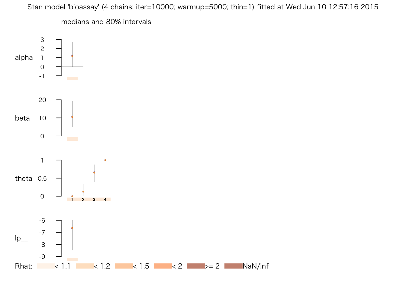
シミュレートされた \(\alpha\) と \(\beta\) を散布図にしてみよう。
Bio.post <- data.frame(alpha = extract(bio.fit.2, "alpha")$alpha,
                       beta = extract(bio.fit.2, "beta")$beta)
bio.scat <- ggplot(sample_n(Bio.post, 1000), aes(x = alpha, y = beta)) +
    geom_point() +
    xlim(-5, 10) + ylim(-10, 40) +
    ggtitle("1000 draws from the posterior simulated by Stan")
print(bio.scat)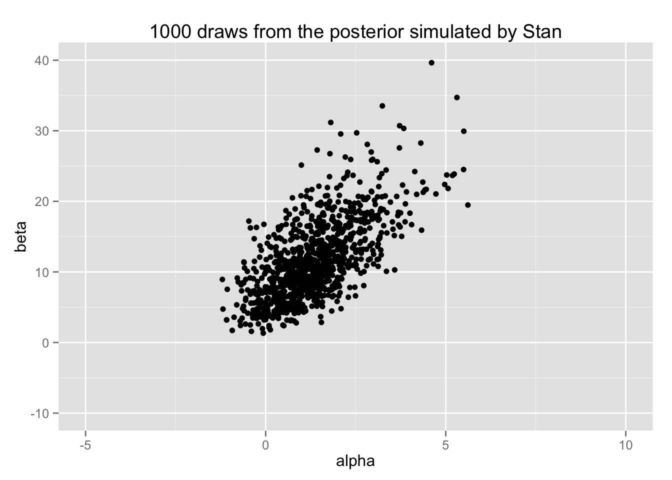
これを BDA3の図3.3 (b) (p.76) と比較せよ。
また、LD50 の分布は、次のようになる。
bio.ld50 <- ggplot(subset(Bio.post, beta > 0), aes(x = -alpha / beta)) +
    geom_histogram(aes(y = ..density..), binwidth = .025)
bio.ld50 + xlab("LD50") +
    ggtitle("Posterior distribution of the LD50 simulated by Stan")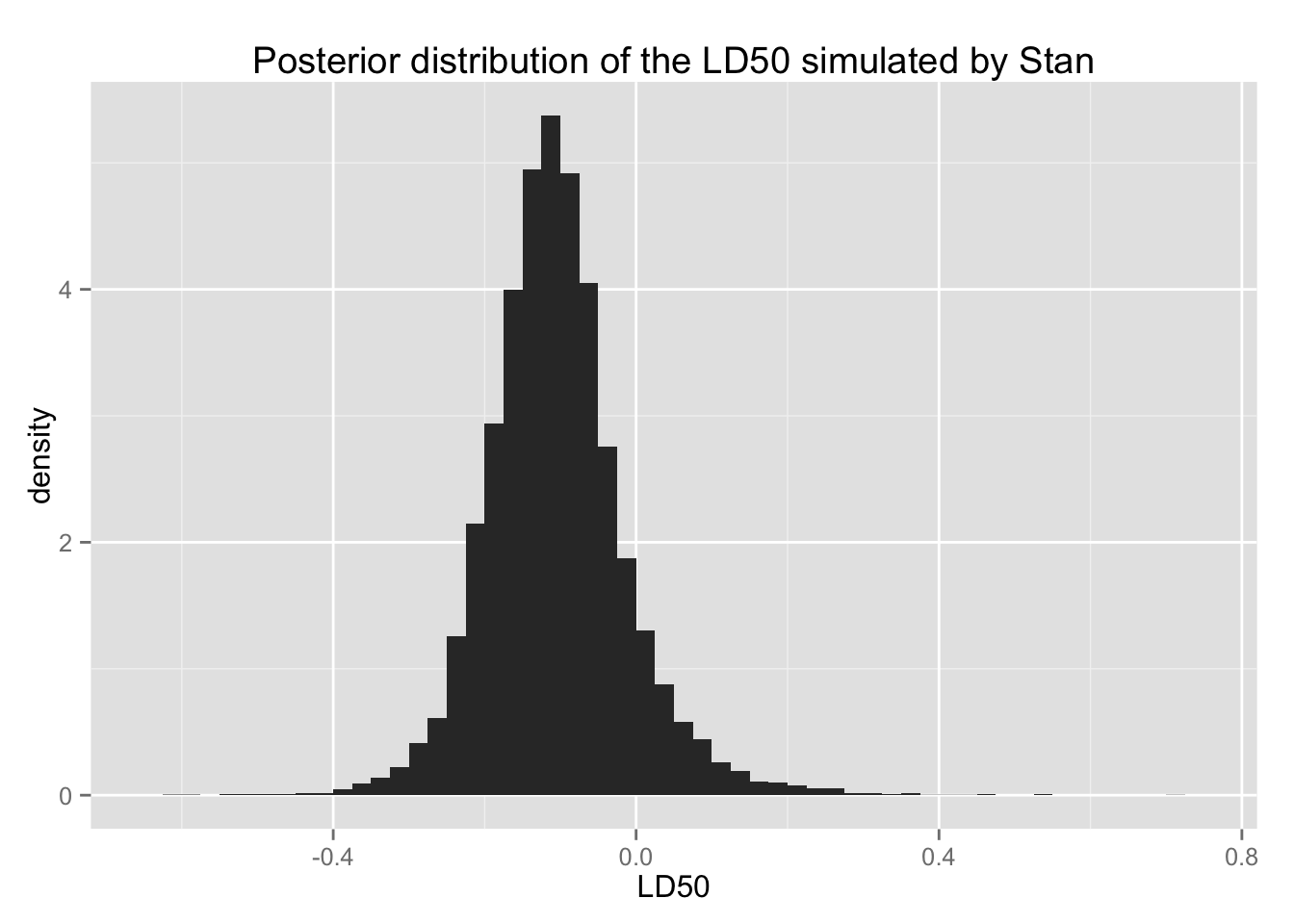
LD50の事後分布を要約する。
Bio.post %>%
    subset(beta > 0) %>%
    mutate(ld50 = -alpha / beta) %>%
    with(quantile(ld50, c(.025, .25, .5, .75, .975)))
## 2.5% 25% 50% 75% 97.5%
## -0.27494370 -0.16076704 -0.11057696 -0.05861233 0.09609832ネズミの腫瘍実験
Stan で推定するために、推定モデルを .stan ファイルに記述する。 ここでは、rat-tumor-2.stan にモデルが記述されている。 このファイルの中身は、以下のとおりである。
data {
    int<lower=1> J;
    int<lower=0> y[J];
    int<lower=1> n[J];
}
parameters {
    real<lower=0, upper=1> theta[J];
    real phi1;
    real phi2;
}
transformed parameters {
    real<lower=0> alpha;
    real<lower=0> beta;
    alpha <- exp(phi1 + phi2) / (1 + exp(phi1));
    beta <- exp(phi2) / (1 + exp(phi1));
}
model {
    theta ~ beta(alpha, beta);
    y ~ binomial(n, theta);
}使用するデータ を読み込み、リストにする。
Rats <- read.table("rats.asc", skip = 3, header = TRUE)
Rats <- list(y = Rats$y, n = Rats$N, J = nrow(Rats))
Stan で推定する。
rat.fit.1 <- stan(file = "rat-tumor-2.stan", data = Rats,
                  iter = 1000, chains = 4)
##
## TRANSLATING MODEL 'rat-tumor-2' FROM Stan CODE TO C++ CODE NOW.
## COMPILING THE C++ CODE FOR MODEL 'rat-tumor-2' NOW.
##
## SAMPLING FOR MODEL 'rat-tumor-2' NOW (CHAIN 1).
##
## Iteration: 1 / 1000 [ 0%] (Warmup)
## Iteration: 100 / 1000 [ 10%] (Warmup)
## Iteration: 200 / 1000 [ 20%] (Warmup)
## Iteration: 300 / 1000 [ 30%] (Warmup)
## Iteration: 400 / 1000 [ 40%] (Warmup)
## Iteration: 500 / 1000 [ 50%] (Warmup)
## Iteration: 501 / 1000 [ 50%] (Sampling)
## Iteration: 600 / 1000 [ 60%] (Sampling)
## Iteration: 700 / 1000 [ 70%] (Sampling)
## Iteration: 800 / 1000 [ 80%] (Sampling)
## Iteration: 900 / 1000 [ 90%] (Sampling)
## Iteration: 1000 / 1000 [100%] (Sampling)
## # Elapsed Time: 0.213909 seconds (Warm-up)
## # 0.168071 seconds (Sampling)
## # 0.38198 seconds (Total)
##
##
## SAMPLING FOR MODEL 'rat-tumor-2' NOW (CHAIN 2).
##
## Iteration: 1 / 1000 [ 0%] (Warmup)
## Iteration: 100 / 1000 [ 10%] (Warmup)
## Iteration: 200 / 1000 [ 20%] (Warmup)
## Iteration: 300 / 1000 [ 30%] (Warmup)
## Iteration: 400 / 1000 [ 40%] (Warmup)
## Iteration: 500 / 1000 [ 50%] (Warmup)
## Iteration: 501 / 1000 [ 50%] (Sampling)
## Iteration: 600 / 1000 [ 60%] (Sampling)
## Iteration: 700 / 1000 [ 70%] (Sampling)
## Iteration: 800 / 1000 [ 80%] (Sampling)
## Iteration: 900 / 1000 [ 90%] (Sampling)
## Iteration: 1000 / 1000 [100%] (Sampling)
## # Elapsed Time: 0.215689 seconds (Warm-up)
## # 0.195653 seconds (Sampling)
## # 0.411342 seconds (Total)
##
##
## SAMPLING FOR MODEL 'rat-tumor-2' NOW (CHAIN 3).
##
## Iteration: 1 / 1000 [ 0%] (Warmup)
## Iteration: 100 / 1000 [ 10%] (Warmup)
## Iteration: 200 / 1000 [ 20%] (Warmup)
## Iteration: 300 / 1000 [ 30%] (Warmup)
## Iteration: 400 / 1000 [ 40%] (Warmup)
## Iteration: 500 / 1000 [ 50%] (Warmup)
## Iteration: 501 / 1000 [ 50%] (Sampling)
## Iteration: 600 / 1000 [ 60%] (Sampling)
## Iteration: 700 / 1000 [ 70%] (Sampling)
## Iteration: 800 / 1000 [ 80%] (Sampling)
## Iteration: 900 / 1000 [ 90%] (Sampling)
## Iteration: 1000 / 1000 [100%] (Sampling)
## # Elapsed Time: 0.250272 seconds (Warm-up)
## # 0.158517 seconds (Sampling)
## # 0.408789 seconds (Total)
##
##
## SAMPLING FOR MODEL 'rat-tumor-2' NOW (CHAIN 4).
##
## Iteration: 1 / 1000 [ 0%] (Warmup)
## Iteration: 100 / 1000 [ 10%] (Warmup)
## Iteration: 200 / 1000 [ 20%] (Warmup)
## Iteration: 300 / 1000 [ 30%] (Warmup)
## Iteration: 400 / 1000 [ 40%] (Warmup)
## Iteration: 500 / 1000 [ 50%] (Warmup)
## Iteration: 501 / 1000 [ 50%] (Sampling)
## Iteration: 600 / 1000 [ 60%] (Sampling)
## Iteration: 700 / 1000 [ 70%] (Sampling)
## Iteration: 800 / 1000 [ 80%] (Sampling)
## Iteration: 900 / 1000 [ 90%] (Sampling)
## Iteration: 1000 / 1000 [100%] (Sampling)
## # Elapsed Time: 0.238442 seconds (Warm-up)
## # 0.179021 seconds (Sampling)
## # 0.417463 seconds (Total)シミュレーションの回数を増やす。
rat.fit.2 <- stan(fit = rat.fit.1, data = Rats, iter = 10000, chains = 4)##
## SAMPLING FOR MODEL 'rat-tumor-2' NOW (CHAIN 1).
##
## Iteration: 1 / 10000 [ 0%] (Warmup)
## Iteration: 1000 / 10000 [ 10%] (Warmup)
## Iteration: 2000 / 10000 [ 20%] (Warmup)
## Iteration: 3000 / 10000 [ 30%] (Warmup)
## Iteration: 4000 / 10000 [ 40%] (Warmup)
## Iteration: 5000 / 10000 [ 50%] (Warmup)
## Iteration: 5001 / 10000 [ 50%] (Sampling)
## Iteration: 6000 / 10000 [ 60%] (Sampling)
## Iteration: 7000 / 10000 [ 70%] (Sampling)
## Iteration: 8000 / 10000 [ 80%] (Sampling)
## Iteration: 9000 / 10000 [ 90%] (Sampling)
## Iteration: 10000 / 10000 [100%] (Sampling)
## # Elapsed Time: 1.42754 seconds (Warm-up)
## # 1.56963 seconds (Sampling)
## # 2.99718 seconds (Total)
##
##
## SAMPLING FOR MODEL 'rat-tumor-2' NOW (CHAIN 2).
##
## Iteration: 1 / 10000 [ 0%] (Warmup)
## Iteration: 1000 / 10000 [ 10%] (Warmup)
## Iteration: 2000 / 10000 [ 20%] (Warmup)
## Iteration: 3000 / 10000 [ 30%] (Warmup)
## Iteration: 4000 / 10000 [ 40%] (Warmup)
## Iteration: 5000 / 10000 [ 50%] (Warmup)
## Iteration: 5001 / 10000 [ 50%] (Sampling)
## Iteration: 6000 / 10000 [ 60%] (Sampling)
## Iteration: 7000 / 10000 [ 70%] (Sampling)
## Iteration: 8000 / 10000 [ 80%] (Sampling)
## Iteration: 9000 / 10000 [ 90%] (Sampling)
## Iteration: 10000 / 10000 [100%] (Sampling)
## # Elapsed Time: 1.41494 seconds (Warm-up)
## # 2.09326 seconds (Sampling)
## # 3.5082 seconds (Total)
##
##
## SAMPLING FOR MODEL 'rat-tumor-2' NOW (CHAIN 3).
##
## Iteration: 1 / 10000 [ 0%] (Warmup)
## Iteration: 1000 / 10000 [ 10%] (Warmup)
## Iteration: 2000 / 10000 [ 20%] (Warmup)
## Iteration: 3000 / 10000 [ 30%] (Warmup)
## Iteration: 4000 / 10000 [ 40%] (Warmup)
## Iteration: 5000 / 10000 [ 50%] (Warmup)
## Iteration: 5001 / 10000 [ 50%] (Sampling)
## Iteration: 6000 / 10000 [ 60%] (Sampling)
## Iteration: 7000 / 10000 [ 70%] (Sampling)
## Iteration: 8000 / 10000 [ 80%] (Sampling)
## Iteration: 9000 / 10000 [ 90%] (Sampling)
## Iteration: 10000 / 10000 [100%] (Sampling)
## # Elapsed Time: 1.4422 seconds (Warm-up)
## # 2.1347 seconds (Sampling)
## # 3.5769 seconds (Total)
##
##
## SAMPLING FOR MODEL 'rat-tumor-2' NOW (CHAIN 4).
##
## Iteration: 1 / 10000 [ 0%] (Warmup)
## Iteration: 1000 / 10000 [ 10%] (Warmup)
## Iteration: 2000 / 10000 [ 20%] (Warmup)
## Iteration: 3000 / 10000 [ 30%] (Warmup)
## Iteration: 4000 / 10000 [ 40%] (Warmup)
## Iteration: 5000 / 10000 [ 50%] (Warmup)
## Iteration: 5001 / 10000 [ 50%] (Sampling)
## Iteration: 6000 / 10000 [ 60%] (Sampling)
## Iteration: 7000 / 10000 [ 70%] (Sampling)
## Iteration: 8000 / 10000 [ 80%] (Sampling)
## Iteration: 9000 / 10000 [ 90%] (Sampling)
## Iteration: 10000 / 10000 [100%] (Sampling)
## # Elapsed Time: 1.60327 seconds (Warm-up)
## # 1.26533 seconds (Sampling)
## # 2.8686 seconds (Total)print(rat.fit.2)## Inference for Stan model: rat-tumor-2.
## 4 chains, each with iter=10000; warmup=5000; thin=1;
## post-warmup draws per chain=5000, total post-warmup draws=20000.
##
## mean se_mean sd 2.5% 25% 50% 75% 97.5%
## theta[1] 0.06 0.00 0.04 0.01 0.03 0.06 0.09 0.16
## theta[2] 0.06 0.00 0.04 0.01 0.03 0.06 0.09 0.16
## theta[3] 0.06 0.00 0.04 0.01 0.03 0.06 0.09 0.16
## theta[4] 0.06 0.00 0.04 0.01 0.03 0.06 0.09 0.16
## theta[5] 0.06 0.00 0.04 0.01 0.03 0.06 0.09 0.16
## theta[6] 0.06 0.00 0.04 0.01 0.03 0.06 0.09 0.17
## theta[7] 0.06 0.00 0.04 0.01 0.03 0.06 0.09 0.17
## theta[8] 0.07 0.00 0.04 0.01 0.03 0.06 0.09 0.17
## theta[9] 0.07 0.00 0.04 0.01 0.03 0.06 0.09 0.17
## theta[10] 0.07 0.00 0.04 0.01 0.03 0.06 0.09 0.17
## theta[11] 0.07 0.00 0.04 0.01 0.03 0.06 0.09 0.17
## theta[12] 0.07 0.00 0.04 0.01 0.04 0.06 0.09 0.17
## theta[13] 0.07 0.00 0.04 0.01 0.04 0.06 0.09 0.17
## theta[14] 0.07 0.00 0.04 0.01 0.04 0.06 0.10 0.18
## theta[15] 0.09 0.00 0.05 0.02 0.06 0.08 0.12 0.20
## theta[16] 0.09 0.00 0.05 0.02 0.06 0.08 0.12 0.20
## theta[17] 0.09 0.00 0.05 0.02 0.06 0.08 0.12 0.21
## theta[18] 0.09 0.00 0.05 0.02 0.06 0.09 0.12 0.20
## theta[19] 0.09 0.00 0.05 0.02 0.06 0.09 0.12 0.21
## theta[20] 0.09 0.00 0.05 0.02 0.06 0.09 0.12 0.21
## theta[21] 0.10 0.00 0.05 0.02 0.06 0.09 0.13 0.21
## theta[22] 0.10 0.00 0.05 0.02 0.06 0.09 0.13 0.21
## theta[23] 0.12 0.00 0.05 0.04 0.09 0.12 0.15 0.23
## theta[24] 0.10 0.00 0.05 0.03 0.07 0.10 0.13 0.21
## theta[25] 0.11 0.00 0.05 0.03 0.07 0.10 0.14 0.22
## theta[26] 0.11 0.00 0.05 0.03 0.07 0.10 0.14 0.22
## theta[27] 0.12 0.00 0.05 0.04 0.08 0.11 0.15 0.24
## theta[28] 0.12 0.00 0.05 0.04 0.08 0.11 0.15 0.24
## theta[29] 0.12 0.00 0.05 0.04 0.08 0.11 0.15 0.24
## theta[30] 0.12 0.00 0.05 0.04 0.08 0.11 0.15 0.24
## theta[31] 0.12 0.00 0.05 0.04 0.08 0.11 0.15 0.24
## theta[32] 0.12 0.00 0.05 0.04 0.08 0.11 0.15 0.24
## theta[33] 0.13 0.00 0.06 0.03 0.08 0.12 0.16 0.28
## theta[34] 0.11 0.00 0.04 0.05 0.08 0.11 0.14 0.20
## theta[35] 0.12 0.00 0.06 0.04 0.08 0.12 0.16 0.25
## theta[36] 0.12 0.00 0.04 0.05 0.09 0.11 0.14 0.21
## theta[37] 0.13 0.00 0.06 0.04 0.09 0.12 0.16 0.26
## theta[38] 0.14 0.00 0.04 0.07 0.11 0.14 0.17 0.24
## theta[39] 0.15 0.00 0.04 0.07 0.12 0.14 0.17 0.24
## theta[40] 0.15 0.00 0.06 0.05 0.10 0.14 0.18 0.28
## theta[41] 0.15 0.00 0.06 0.05 0.10 0.14 0.18 0.28
## theta[42] 0.15 0.00 0.07 0.05 0.10 0.14 0.19 0.30
## theta[43] 0.18 0.00 0.05 0.09 0.14 0.17 0.21 0.28
## theta[44] 0.19 0.00 0.05 0.10 0.15 0.18 0.22 0.29
## theta[45] 0.17 0.00 0.06 0.07 0.13 0.17 0.21 0.31
## theta[46] 0.17 0.00 0.06 0.07 0.13 0.17 0.21 0.31
## theta[47] 0.17 0.00 0.06 0.07 0.13 0.17 0.21 0.31
## theta[48] 0.17 0.00 0.06 0.07 0.13 0.17 0.21 0.31
## theta[49] 0.17 0.00 0.06 0.07 0.13 0.17 0.21 0.31
## theta[50] 0.17 0.00 0.06 0.07 0.13 0.17 0.21 0.31
## theta[51] 0.17 0.00 0.06 0.07 0.13 0.17 0.21 0.32
## theta[52] 0.19 0.00 0.05 0.10 0.16 0.19 0.22 0.30
## theta[53] 0.18 0.00 0.06 0.07 0.13 0.17 0.22 0.32
## theta[54] 0.18 0.00 0.07 0.07 0.13 0.17 0.22 0.32
## theta[55] 0.18 0.00 0.06 0.07 0.13 0.17 0.22 0.32
## theta[56] 0.19 0.00 0.06 0.09 0.15 0.19 0.23 0.33
## theta[57] 0.21 0.00 0.05 0.12 0.18 0.21 0.25 0.33
## theta[58] 0.22 0.00 0.05 0.13 0.18 0.22 0.25 0.33
## theta[59] 0.20 0.00 0.07 0.09 0.15 0.20 0.24 0.35
## theta[60] 0.20 0.00 0.07 0.09 0.15 0.19 0.24 0.35
## theta[61] 0.21 0.00 0.07 0.10 0.16 0.21 0.25 0.35
## theta[62] 0.21 0.00 0.07 0.09 0.16 0.20 0.25 0.36
## theta[63] 0.22 0.00 0.07 0.10 0.17 0.21 0.26 0.36
## theta[64] 0.23 0.00 0.07 0.11 0.18 0.22 0.27 0.38
## theta[65] 0.23 0.00 0.07 0.11 0.18 0.22 0.27 0.38
## theta[66] 0.23 0.00 0.07 0.11 0.18 0.22 0.27 0.38
## theta[67] 0.27 0.00 0.05 0.17 0.23 0.27 0.30 0.38
## theta[68] 0.28 0.00 0.06 0.17 0.24 0.27 0.31 0.39
## theta[69] 0.27 0.00 0.06 0.17 0.23 0.27 0.31 0.39
## theta[70] 0.28 0.00 0.07 0.15 0.23 0.28 0.33 0.44
## theta[71] 0.21 0.00 0.07 0.08 0.15 0.20 0.25 0.37
## phi1 -1.80 0.00 0.11 -2.01 -1.87 -1.79 -1.72 -1.59
## phi2 2.80 0.01 0.35 2.15 2.56 2.79 3.03 3.53
## alpha 2.50 0.02 0.97 1.23 1.84 2.31 2.93 4.88
## beta 15.06 0.12 5.81 7.35 11.12 13.95 17.71 29.21
## lp__ -781.93 0.22 9.66 -801.29 -788.33 -781.74 -775.44 -763.58
## n_eff Rhat
## theta[1] 20000 1
## theta[2] 20000 1
## theta[3] 20000 1
## theta[4] 20000 1
## theta[5] 20000 1
## theta[6] 20000 1
## theta[7] 20000 1
## theta[8] 20000 1
## theta[9] 20000 1
## theta[10] 20000 1
## theta[11] 20000 1
## theta[12] 20000 1
## theta[13] 20000 1
## theta[14] 20000 1
## theta[15] 20000 1
## theta[16] 20000 1
## theta[17] 20000 1
## theta[18] 20000 1
## theta[19] 20000 1
## theta[20] 20000 1
## theta[21] 20000 1
## theta[22] 20000 1
## theta[23] 20000 1
## theta[24] 20000 1
## theta[25] 20000 1
## theta[26] 20000 1
## theta[27] 20000 1
## theta[28] 20000 1
## theta[29] 20000 1
## theta[30] 20000 1
## theta[31] 20000 1
## theta[32] 20000 1
## theta[33] 20000 1
## theta[34] 20000 1
## theta[35] 20000 1
## theta[36] 20000 1
## theta[37] 20000 1
## theta[38] 20000 1
## theta[39] 20000 1
## theta[40] 20000 1
## theta[41] 20000 1
## theta[42] 20000 1
## theta[43] 20000 1
## theta[44] 20000 1
## theta[45] 20000 1
## theta[46] 20000 1
## theta[47] 20000 1
## theta[48] 20000 1
## theta[49] 20000 1
## theta[50] 20000 1
## theta[51] 20000 1
## theta[52] 20000 1
## theta[53] 20000 1
## theta[54] 20000 1
## theta[55] 20000 1
## theta[56] 20000 1
## theta[57] 20000 1
## theta[58] 20000 1
## theta[59] 20000 1
## theta[60] 20000 1
## theta[61] 20000 1
## theta[62] 20000 1
## theta[63] 20000 1
## theta[64] 20000 1
## theta[65] 20000 1
## theta[66] 20000 1
## theta[67] 20000 1
## theta[68] 20000 1
## theta[69] 20000 1
## theta[70] 20000 1
## theta[71] 20000 1
## phi1 13945 1
## phi2 2340 1
## alpha 2048 1
## beta 2192 1
## lp__ 1922 1
##
## Samples were drawn using NUTS(diag_e) at Wed Jun 10 18:55:14 2015.
## For each parameter, n_eff is a crude measure of effective sample size,
## and Rhat is the potential scale reduction factor on split chains (at
## convergence, Rhat=1).plot(rat.fit.2)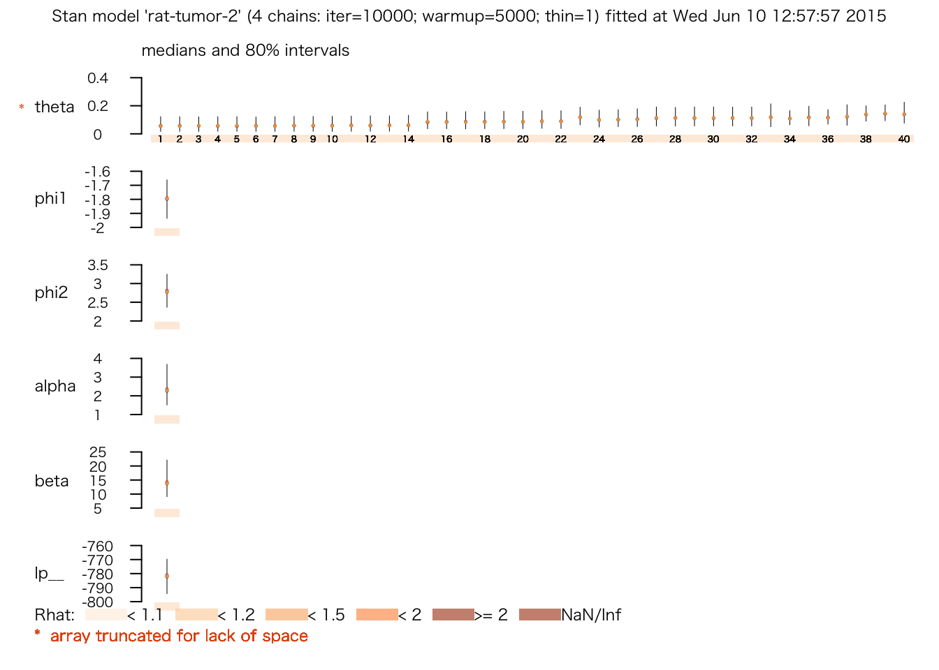
\(\mathrm{log}(\alpha / \beta)\) と\(\mathrm{log}(\alpha + \beta)\) の散布図を描いてみよう。 ここでは、phi1 \(= \mathrm{log}(\alpha / \beta)\), phi2 \(=\mathrm{log}(\alpha + \beta)\) である。
Phi <- data.frame(phi1 = extract(rat.fit.2, "phi1")$phi1,
                  phi2 = extract(rat.fit.2, "phi2")$phi2)
rat.scat <- ggplot(sample_n(Phi, 1000), aes(x = phi1, y = phi2)) +
    geom_point() +
    xlim(-2.2, -1.4) + ylim(1, 5) + coord_fixed(ratio = .2) +
    labs(x = "log(alpha / beta)", y = "log(alpha/beta)",
         title = "1000 draws from Stan simulation")
print(rat.scat)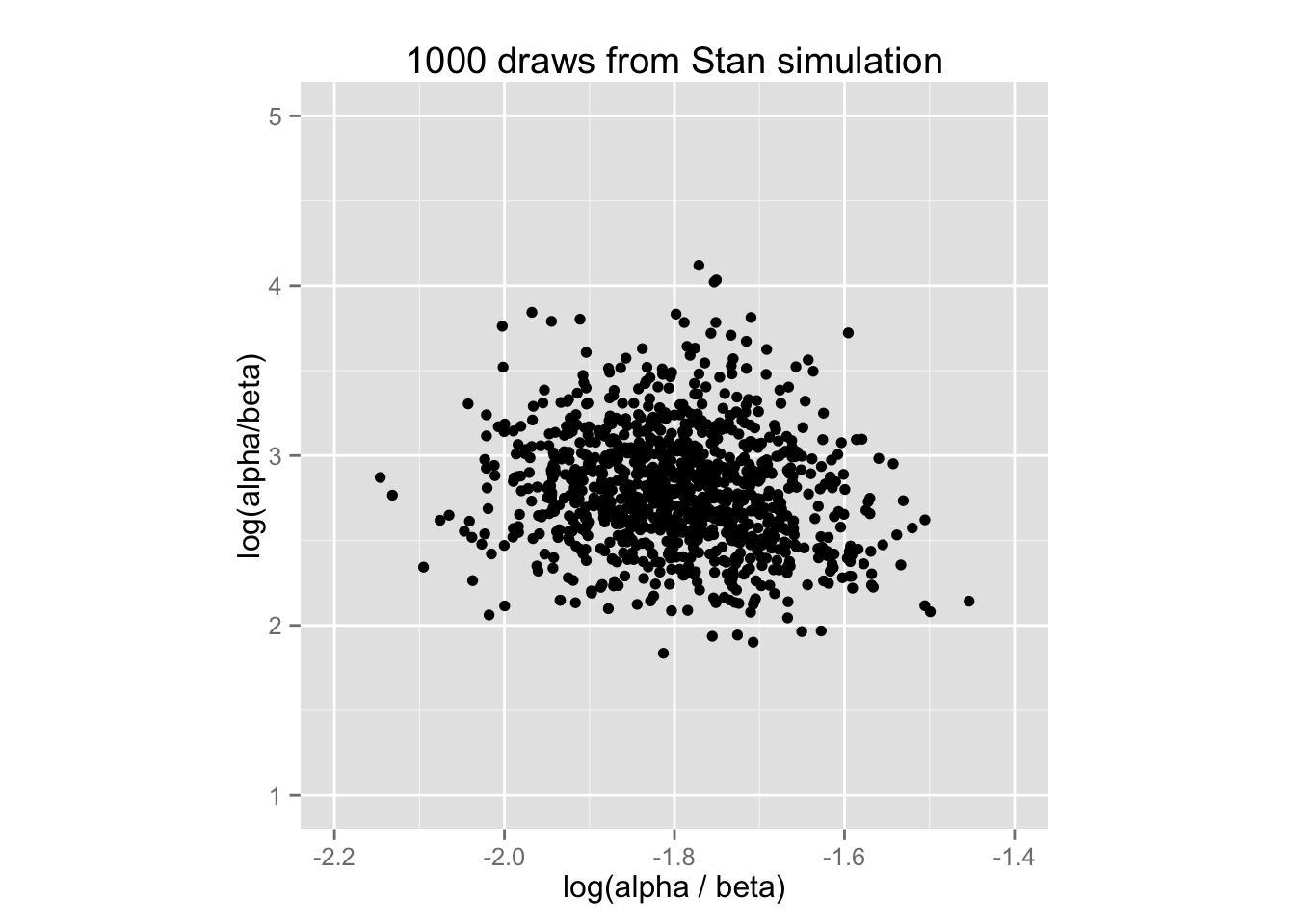
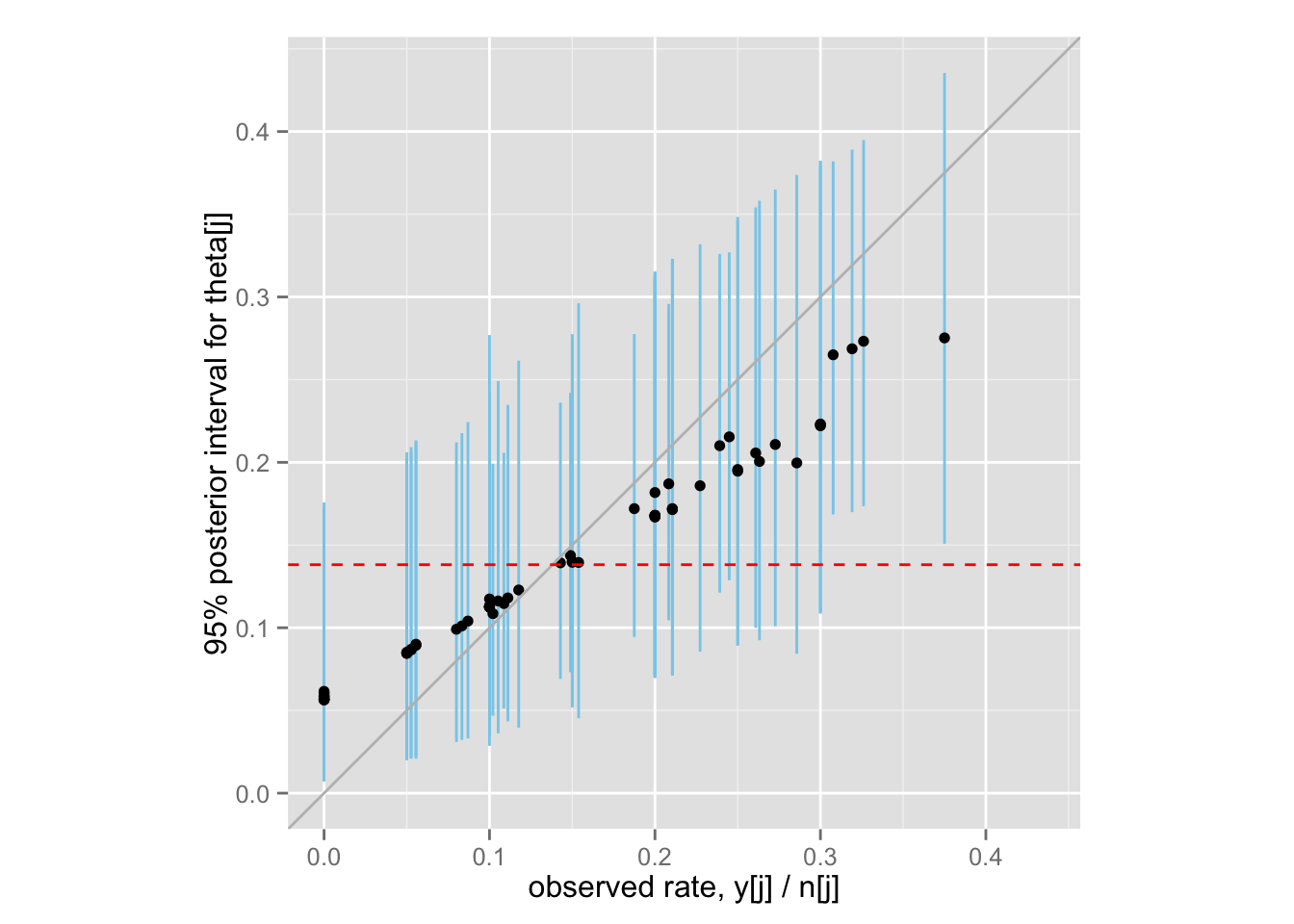
最後に、ベイズ収縮(shrinkage)を示す図5.4 (BDA3, p.113) を再現してみよう。
theta.samples <- extract(rat.fit.2, "theta")$theta
Post <- data.frame(
    rate = Rats$y / Rats$n,
    med = apply(theta.samples, 2, median),
    lower = apply(theta.samples, 2, function(x) quantile(x, .025)),
    upper = apply(theta.samples, 2, function(x) quantile(x, .975))
    )
shrinkage <- ggplot(Post, aes(x = rate, y = med)) +
    geom_linerange(aes(ymin = lower, ymax = upper), color = "skyblue") +
    geom_point() +
    xlim(0, max(Post$upper)) + ylim(0, max(Post$upper)) + coord_fixed() +
    geom_abline(intercept = 0, slope = 1, color = "gray") +
    geom_hline(yintercept = mean(Post$rate), color = "red", linetype = "dashed")
shrinkage + labs(x = "observed rate, y[j] / n[j]",
                 y = "95% posterior interval for theta[j]")