政治学方法論 II:回帰モデル
矢内 勇生
2015年7月22日
準備
library("coefplot")## Loading required package: ggplot2library("rstan")## Loading required package: Rcpp
## Loading required package: inline
##
## Attaching package: 'inline'
##
## The following object is masked from 'package:Rcpp':
##
## registerPlugin
##
## rstan (Version 2.6.0, packaged: 2015-02-06 21:02:34 UTC, GitRev: 198082f07a60)Normal Linear モデル
まず、偽データを作る。
set.seed(2015-07-22)
n <- 50
true_beta <- c(2, 0.2, 1.5, -2)
true_sigma <- 3
x2 <- runif(n, min = 1, max = 10)
x3 <- rnorm(n, mean = 0, sd = 4)
x4 <- runif(n, min = -10, max = 10)
y <- true_beta[1] + true_beta[2] * x2 + true_beta[3] * x3 +
  true_beta[4] * x4 + rnorm(n, mean = 0, sd = true_sigma)
通常の回帰分析を行う。
fit.1 <- lm(y ~ x2 + x3 + x4)
summary(fit.1)
##
## Call:
## lm(formula = y ~ x2 + x3 + x4)
##
## Residuals:
## Min 1Q Median 3Q Max
## -5.9244 -2.1057 -0.4294 1.9519 6.6191
##
## Coefficients:
## Estimate Std. Error t value Pr(>|t|)
## (Intercept) 2.70413 1.05834 2.555 0.014
## x2 0.12642 0.17758 0.712 0.480
## x3 1.59030 0.11658 13.642 <2e-16
## x4 -1.95201 0.07909 -24.680 <2e-16
##
## Residual standard error: 2.951 on 46 degrees of freedom
## Multiple R-squared: 0.9355, Adjusted R-squared: 0.9313
## F-statistic: 222.3 on 3 and 46 DF, p-value: < 2.2e-16推定結果をキャタピラプロットで示す。
coefplot(fit.1, intercept = TRUE)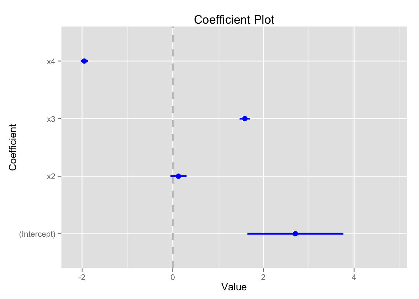
次に、Stan を使ってベイズ推定する。 Stan モデルは regression-1.stan を使う。
Fake.1 <- list(N = n, y = y, x2 = x2, x3 = x3, x4 = x4)
fit.2 <- stan(file = "regression-1.stan", data = Fake.1, iter = 1000, chains = 4)
##
## TRANSLATING MODEL 'regression-1' FROM Stan CODE TO C++ CODE NOW.
## COMPILING THE C++ CODE FOR MODEL 'regression-1' NOW.
##
## SAMPLING FOR MODEL 'regression-1' NOW (CHAIN 1).
##
## Iteration: 1 / 1000 [ 0%] (Warmup)
## Iteration: 100 / 1000 [ 10%] (Warmup)
## Iteration: 200 / 1000 [ 20%] (Warmup)
## Iteration: 300 / 1000 [ 30%] (Warmup)
## Iteration: 400 / 1000 [ 40%] (Warmup)
## Iteration: 500 / 1000 [ 50%] (Warmup)
## Iteration: 501 / 1000 [ 50%] (Sampling)
## Iteration: 600 / 1000 [ 60%] (Sampling)
## Iteration: 700 / 1000 [ 70%] (Sampling)
## Iteration: 800 / 1000 [ 80%] (Sampling)
## Iteration: 900 / 1000 [ 90%] (Sampling)
## Iteration: 1000 / 1000 [100%] (Sampling)
## # Elapsed Time: 0.040991 seconds (Warm-up)
## # 0.038335 seconds (Sampling)
## # 0.079326 seconds (Total)
##
##
## SAMPLING FOR MODEL 'regression-1' NOW (CHAIN 2).
##
## Iteration: 1 / 1000 [ 0%] (Warmup)
## Iteration: 100 / 1000 [ 10%] (Warmup)
## Iteration: 200 / 1000 [ 20%] (Warmup)
## Iteration: 300 / 1000 [ 30%] (Warmup)
## Iteration: 400 / 1000 [ 40%] (Warmup)
## Iteration: 500 / 1000 [ 50%] (Warmup)
## Iteration: 501 / 1000 [ 50%] (Sampling)
## Iteration: 600 / 1000 [ 60%] (Sampling)
## Iteration: 700 / 1000 [ 70%] (Sampling)
## Iteration: 800 / 1000 [ 80%] (Sampling)
## Iteration: 900 / 1000 [ 90%] (Sampling)
## Iteration: 1000 / 1000 [100%] (Sampling)
## # Elapsed Time: 0.042831 seconds (Warm-up)
## # 0.036998 seconds (Sampling)
## # 0.079829 seconds (Total)
##
##
## SAMPLING FOR MODEL 'regression-1' NOW (CHAIN 3).
##
## Iteration: 1 / 1000 [ 0%] (Warmup)
## Iteration: 100 / 1000 [ 10%] (Warmup)
## Iteration: 200 / 1000 [ 20%] (Warmup)
## Iteration: 300 / 1000 [ 30%] (Warmup)
## Iteration: 400 / 1000 [ 40%] (Warmup)
## Iteration: 500 / 1000 [ 50%] (Warmup)
## Iteration: 501 / 1000 [ 50%] (Sampling)
## Iteration: 600 / 1000 [ 60%] (Sampling)
## Iteration: 700 / 1000 [ 70%] (Sampling)
## Iteration: 800 / 1000 [ 80%] (Sampling)
## Iteration: 900 / 1000 [ 90%] (Sampling)
## Iteration: 1000 / 1000 [100%] (Sampling)
## # Elapsed Time: 0.038978 seconds (Warm-up)
## # 0.037026 seconds (Sampling)
## # 0.076004 seconds (Total)
##
##
## SAMPLING FOR MODEL 'regression-1' NOW (CHAIN 4).
##
## Iteration: 1 / 1000 [ 0%] (Warmup)
## Iteration: 100 / 1000 [ 10%] (Warmup)
## Iteration: 200 / 1000 [ 20%] (Warmup)
## Iteration: 300 / 1000 [ 30%] (Warmup)
## Iteration: 400 / 1000 [ 40%] (Warmup)
## Iteration: 500 / 1000 [ 50%] (Warmup)
## Iteration: 501 / 1000 [ 50%] (Sampling)
## Iteration: 600 / 1000 [ 60%] (Sampling)
## Iteration: 700 / 1000 [ 70%] (Sampling)
## Iteration: 800 / 1000 [ 80%] (Sampling)
## Iteration: 900 / 1000 [ 90%] (Sampling)
## Iteration: 1000 / 1000 [100%] (Sampling)
## # Elapsed Time: 0.037115 seconds (Warm-up)
## # 0.040262 seconds (Sampling)
## # 0.077377 seconds (Total)fit.2.upd <- stan(fit = fit.2, data = Fake.1, iter = 10000, chains = 4)##
## SAMPLING FOR MODEL 'regression-1' NOW (CHAIN 1).
##
## Iteration: 1 / 10000 [ 0%] (Warmup)
## Iteration: 1000 / 10000 [ 10%] (Warmup)
## Iteration: 2000 / 10000 [ 20%] (Warmup)
## Iteration: 3000 / 10000 [ 30%] (Warmup)
## Iteration: 4000 / 10000 [ 40%] (Warmup)
## Iteration: 5000 / 10000 [ 50%] (Warmup)
## Iteration: 5001 / 10000 [ 50%] (Sampling)
## Iteration: 6000 / 10000 [ 60%] (Sampling)
## Iteration: 7000 / 10000 [ 70%] (Sampling)
## Iteration: 8000 / 10000 [ 80%] (Sampling)
## Iteration: 9000 / 10000 [ 90%] (Sampling)
## Iteration: 10000 / 10000 [100%] (Sampling)
## # Elapsed Time: 0.318399 seconds (Warm-up)
## # 0.398944 seconds (Sampling)
## # 0.717343 seconds (Total)
##
##
## SAMPLING FOR MODEL 'regression-1' NOW (CHAIN 2).
##
## Iteration: 1 / 10000 [ 0%] (Warmup)
## Iteration: 1000 / 10000 [ 10%] (Warmup)
## Iteration: 2000 / 10000 [ 20%] (Warmup)
## Iteration: 3000 / 10000 [ 30%] (Warmup)
## Iteration: 4000 / 10000 [ 40%] (Warmup)
## Iteration: 5000 / 10000 [ 50%] (Warmup)
## Iteration: 5001 / 10000 [ 50%] (Sampling)
## Iteration: 6000 / 10000 [ 60%] (Sampling)
## Iteration: 7000 / 10000 [ 70%] (Sampling)
## Iteration: 8000 / 10000 [ 80%] (Sampling)
## Iteration: 9000 / 10000 [ 90%] (Sampling)
## Iteration: 10000 / 10000 [100%] (Sampling)
## # Elapsed Time: 0.295952 seconds (Warm-up)
## # 0.326371 seconds (Sampling)
## # 0.622323 seconds (Total)
##
##
## SAMPLING FOR MODEL 'regression-1' NOW (CHAIN 3).
##
## Iteration: 1 / 10000 [ 0%] (Warmup)
## Iteration: 1000 / 10000 [ 10%] (Warmup)
## Iteration: 2000 / 10000 [ 20%] (Warmup)
## Iteration: 3000 / 10000 [ 30%] (Warmup)
## Iteration: 4000 / 10000 [ 40%] (Warmup)
## Iteration: 5000 / 10000 [ 50%] (Warmup)
## Iteration: 5001 / 10000 [ 50%] (Sampling)
## Iteration: 6000 / 10000 [ 60%] (Sampling)
## Iteration: 7000 / 10000 [ 70%] (Sampling)
## Iteration: 8000 / 10000 [ 80%] (Sampling)
## Iteration: 9000 / 10000 [ 90%] (Sampling)
## Iteration: 10000 / 10000 [100%] (Sampling)
## # Elapsed Time: 0.300807 seconds (Warm-up)
## # 0.397016 seconds (Sampling)
## # 0.697823 seconds (Total)
##
##
## SAMPLING FOR MODEL 'regression-1' NOW (CHAIN 4).
##
## Iteration: 1 / 10000 [ 0%] (Warmup)
## Iteration: 1000 / 10000 [ 10%] (Warmup)
## Iteration: 2000 / 10000 [ 20%] (Warmup)
## Iteration: 3000 / 10000 [ 30%] (Warmup)
## Iteration: 4000 / 10000 [ 40%] (Warmup)
## Iteration: 5000 / 10000 [ 50%] (Warmup)
## Iteration: 5001 / 10000 [ 50%] (Sampling)
## Iteration: 6000 / 10000 [ 60%] (Sampling)
## Iteration: 7000 / 10000 [ 70%] (Sampling)
## Iteration: 8000 / 10000 [ 80%] (Sampling)
## Iteration: 9000 / 10000 [ 90%] (Sampling)
## Iteration: 10000 / 10000 [100%] (Sampling)
## # Elapsed Time: 0.322654 seconds (Warm-up)
## # 0.335888 seconds (Sampling)
## # 0.658542 seconds (Total)plot(fit.2.upd)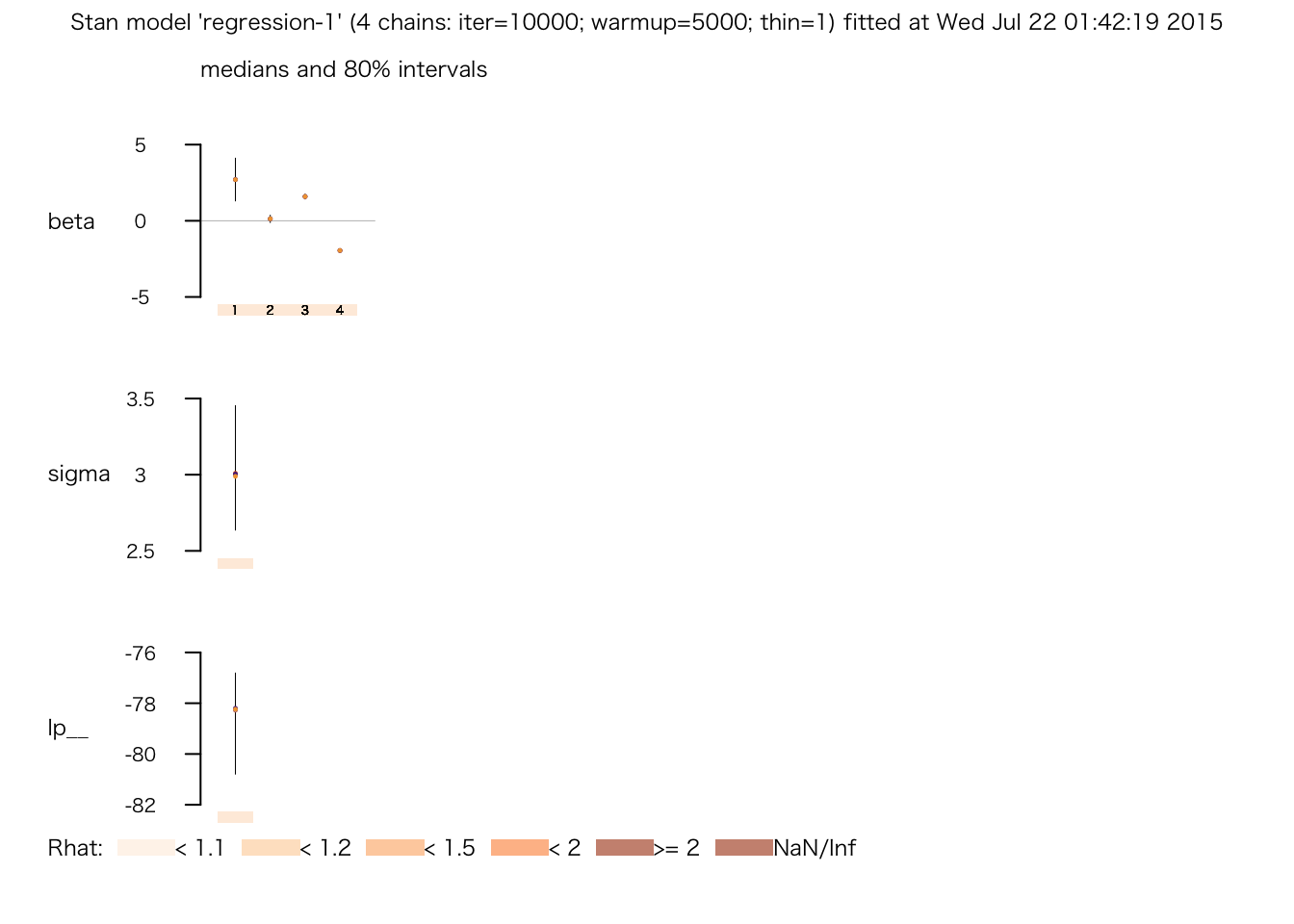
print(fit.2.upd)## Inference for Stan model: regression-1.
## 4 chains, each with iter=10000; warmup=5000; thin=1;
## post-warmup draws per chain=5000, total post-warmup draws=20000.
##
## mean se_mean sd 2.5% 25% 50% 75% 97.5% n_eff Rhat
## beta[1] 2.70 0.01 1.10 0.53 1.97 2.71 3.44 4.84 8266 1
## beta[2] 0.13 0.00 0.18 -0.24 0.00 0.13 0.25 0.50 8338 1
## beta[3] 1.59 0.00 0.12 1.35 1.51 1.59 1.67 1.83 11252 1
## beta[4] -1.95 0.00 0.08 -2.11 -2.01 -1.95 -1.90 -1.79 10356 1
## sigma 3.03 0.00 0.33 2.48 2.80 3.00 3.23 3.75 10201 1
## lp__ -78.58 0.02 1.65 -82.66 -79.43 -78.24 -77.37 -76.41 6332 1
##
## Samples were drawn using NUTS(diag_e) at Wed Jul 22 01:42:19 2015.
## For each parameter, n_eff is a crude measure of effective sample size,
## and Rhat is the potential scale reduction factor on split chains (at
## convergence, Rhat=1).点推定の結果は、通常の回帰分析と同様になることがわかる。
この推定結果を図示する。
post.beta <- extract(fit.2.upd, "beta")$beta
post.sigma <- extract(fit.2.upd, "sigma")$sigma
hist(post.beta[, 1], col = "gray",
     main = expression(paste("Posterior of ", beta[1])))
hist(post.beta[, 2], col = "gray",
     main = expression(paste("Posterior of ", beta[2])))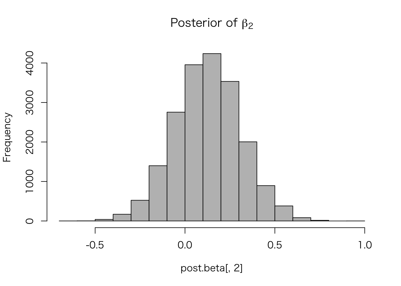
hist(post.beta[, 3], col = "gray",
     main = expression(paste("Posterior of ", beta[3])))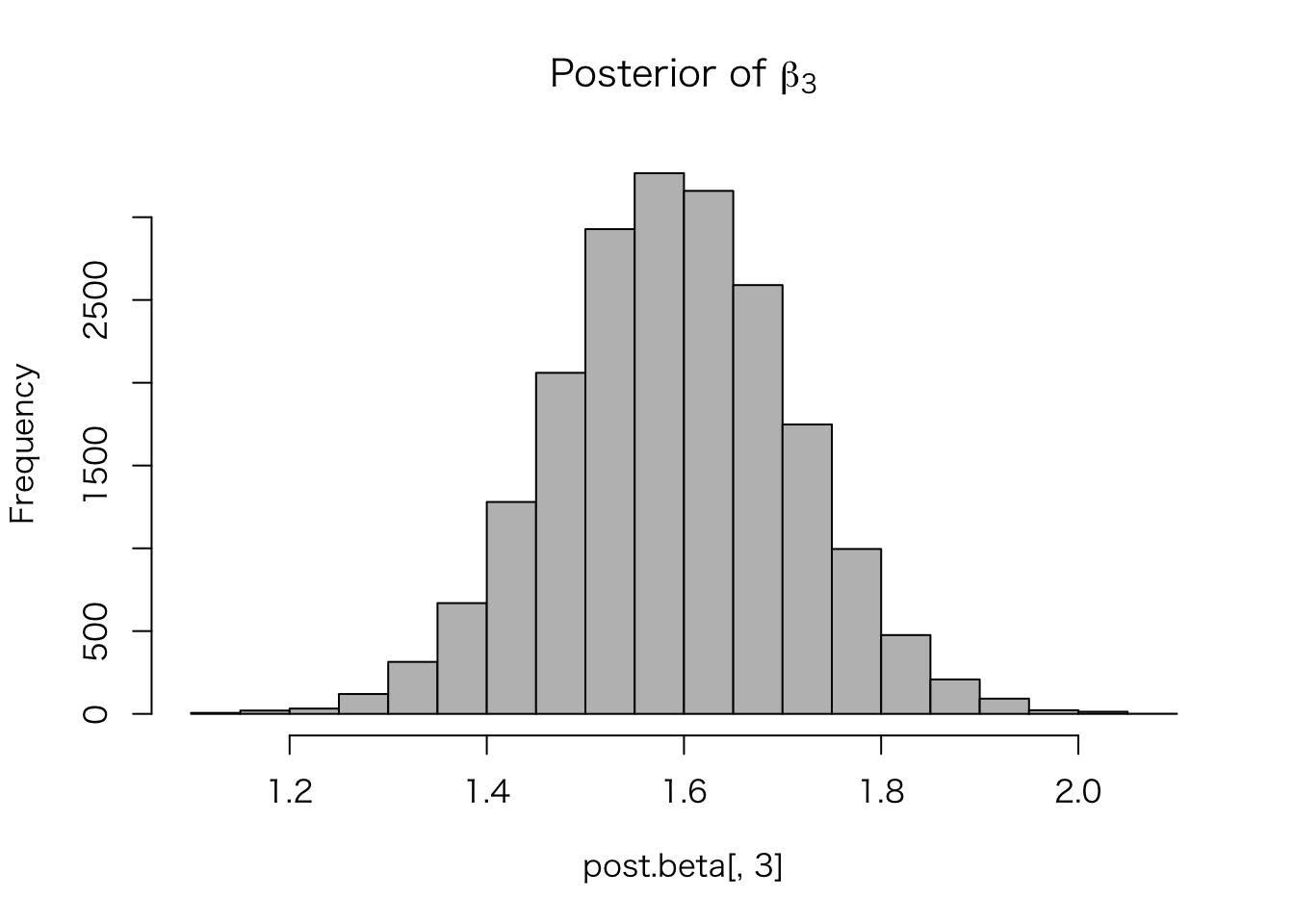
hist(post.beta[, 4], col = "gray",
     main = expression(paste("Posterior of ", beta[4])))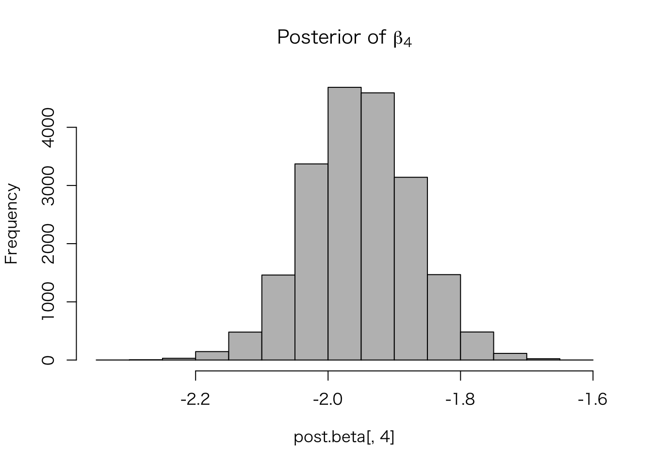
hist(post.sigma, col = "gray",
     main = expression(paste("Posterior of ", sigma)))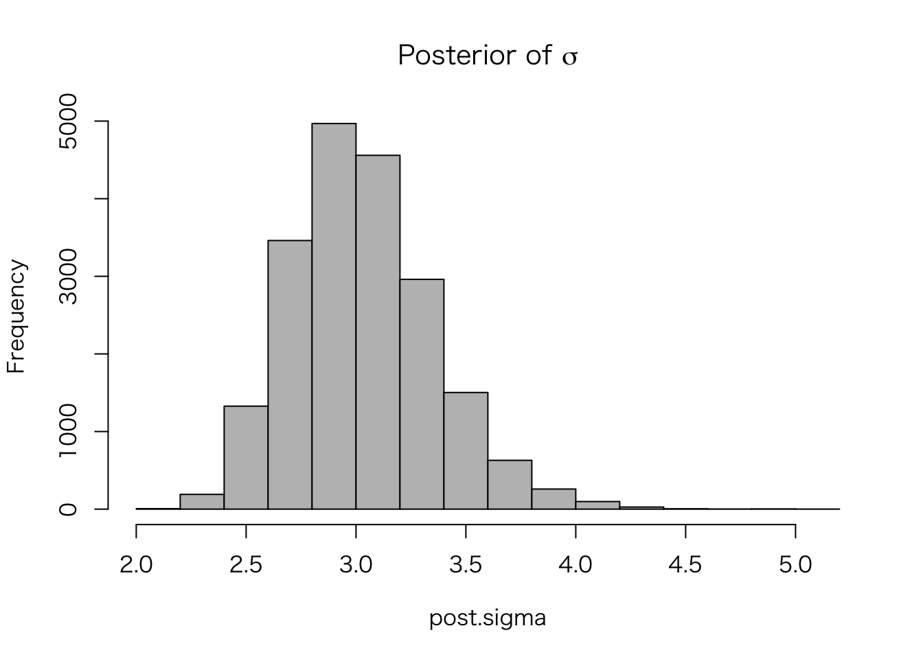
分布が得られるので、求めたい確率を計算することができる。 たとえば、\(\beta_2 | y\) が 0 より大きい確率は、
sum(post.beta[, 2] > 0) / length(post.beta[, 2])## [1] 0.75545である。同様に、\(\sigma | y\) が2.5以上、3.5以下である確率は、
sum(post.sigma >= 2.5 & post.sigma <= 3.5) / length(post.sigma)## [1] 0.88795である。