政治学方法論 II:課題10の解答例
矢内 勇生
2015年6月24日
準備
必要なパッケージを読み込む。インストールの必要があれば各自インストールする。
library("tidyr")
library("dplyr")
library("ggplot2")
library("MCMCpack")
library("pscl")
library("rstan")
問1:打率の推定 正規分布モデル
1-1
打率のおおよその範囲を適当に推測し、95%事前区間を \([0.15, 0.3]\) とする(この区間は各自異なるはず)。
1-2
上で設定した95%事前区間を使うと、その中央値(中間点)は、 \[b_0 = \frac{1}{2}(0.3 - 0.15) + 0.15 = 0.225\] 分散は、 \[B_0 = \left(\frac{0.15}{(2 \cdot 1.96)}\right)^2 \approx 0.0015\] となる。
1-3
モデルを整理すると、次のようになる。
サンプリングモデル: \[y_j | \theta_j \sim \mbox{N}(\theta_j, \sigma^2)\] ただし、\(y_j\) は打率、\[\sigma^2 = \frac{\bar{y}(1-\bar{y})}{n}.\]
事前分布: \[\theta_j | \mu_0, \sigma_0^2 \sim \mbox{N}(\mu_0, \sigma_0^2).\]
超事前分布: \[\mu_0 \sim \mbox{N}(0.225, 0.0015),\] \[\sigma_0^2 \sim \mbox{Inv-Gamma}(7, 0.0175).\]
このモデルをStanモデルとして batting-avg-1.stan に書く。
// batting-avg-1.stan
data {
    int<lower=1> J;
    real<lower=0, upper=1> y[J];
    real<lower=0> sigma;
}
parameters {
    real<lower=0, upper=1> theta[J];
    real<lower=0, upper=1> mu0;
    real<lower=0> sigma0_sq;
}
model {
    mu0 ~ normal(0.225, sqrt(0.0015));    // hyperprior
    sigma0_sq ~ inv_gamma(7, 0.0175);     // hyperprior
    theta ~ normal(mu0, sqrt(sigma0_sq)); // prior
    y ~ normal(theta, sigma);             // likelihood
}
データをリストにする。
data(EfronMorris)
sigma <- with(EfronMorris, sqrt((mean(y) * (1 - mean(y))) / 45))
Bat <- list(J = nrow(EfronMorris),
            y = EfronMorris$y,
            sigma = sigma)
RStan で推定する。
fit.1 <- stan(file = "batting-avg-1.stan", data = Bat, iter = 1000, chains = 4)##
## TRANSLATING MODEL 'batting-avg-1' FROM Stan CODE TO C++ CODE NOW.
## COMPILING THE C++ CODE FOR MODEL 'batting-avg-1' NOW.
##
## SAMPLING FOR MODEL 'batting-avg-1' NOW (CHAIN 1).
##
## Iteration: 1 / 1000 [ 0%] (Warmup)
## Iteration: 100 / 1000 [ 10%] (Warmup)
## Iteration: 200 / 1000 [ 20%] (Warmup)
## Iteration: 300 / 1000 [ 30%] (Warmup)
## Iteration: 400 / 1000 [ 40%] (Warmup)
## Iteration: 500 / 1000 [ 50%] (Warmup)
## Iteration: 501 / 1000 [ 50%] (Sampling)
## Iteration: 600 / 1000 [ 60%] (Sampling)
## Iteration: 700 / 1000 [ 70%] (Sampling)
## Iteration: 800 / 1000 [ 80%] (Sampling)
## Iteration: 900 / 1000 [ 90%] (Sampling)
## Iteration: 1000 / 1000 [100%] (Sampling)
## # Elapsed Time: 0.047026 seconds (Warm-up)
## # 0.032518 seconds (Sampling)
## # 0.079544 seconds (Total)
##
##
## SAMPLING FOR MODEL 'batting-avg-1' NOW (CHAIN 2).
##
## Iteration: 1 / 1000 [ 0%] (Warmup)
## Iteration: 100 / 1000 [ 10%] (Warmup)
## Iteration: 200 / 1000 [ 20%] (Warmup)
## Iteration: 300 / 1000 [ 30%] (Warmup)
## Iteration: 400 / 1000 [ 40%] (Warmup)
## Iteration: 500 / 1000 [ 50%] (Warmup)
## Iteration: 501 / 1000 [ 50%] (Sampling)
## Iteration: 600 / 1000 [ 60%] (Sampling)
## Iteration: 700 / 1000 [ 70%] (Sampling)
## Iteration: 800 / 1000 [ 80%] (Sampling)
## Iteration: 900 / 1000 [ 90%] (Sampling)
## Iteration: 1000 / 1000 [100%] (Sampling)
## # Elapsed Time: 0.046355 seconds (Warm-up)
## # 0.029798 seconds (Sampling)
## # 0.076153 seconds (Total)
##
##
## SAMPLING FOR MODEL 'batting-avg-1' NOW (CHAIN 3).
##
## Iteration: 1 / 1000 [ 0%] (Warmup)
## Iteration: 100 / 1000 [ 10%] (Warmup)
## Iteration: 200 / 1000 [ 20%] (Warmup)
## Iteration: 300 / 1000 [ 30%] (Warmup)
## Iteration: 400 / 1000 [ 40%] (Warmup)
## Iteration: 500 / 1000 [ 50%] (Warmup)
## Iteration: 501 / 1000 [ 50%] (Sampling)
## Iteration: 600 / 1000 [ 60%] (Sampling)
## Iteration: 700 / 1000 [ 70%] (Sampling)
## Iteration: 800 / 1000 [ 80%] (Sampling)
## Iteration: 900 / 1000 [ 90%] (Sampling)
## Iteration: 1000 / 1000 [100%] (Sampling)
## # Elapsed Time: 0.043831 seconds (Warm-up)
## # 0.027596 seconds (Sampling)
## # 0.071427 seconds (Total)
##
##
## SAMPLING FOR MODEL 'batting-avg-1' NOW (CHAIN 4).
##
## Iteration: 1 / 1000 [ 0%] (Warmup)
## Iteration: 100 / 1000 [ 10%] (Warmup)
## Iteration: 200 / 1000 [ 20%] (Warmup)
## Iteration: 300 / 1000 [ 30%] (Warmup)
## Iteration: 400 / 1000 [ 40%] (Warmup)
## Iteration: 500 / 1000 [ 50%] (Warmup)
## Iteration: 501 / 1000 [ 50%] (Sampling)
## Iteration: 600 / 1000 [ 60%] (Sampling)
## Iteration: 700 / 1000 [ 70%] (Sampling)
## Iteration: 800 / 1000 [ 80%] (Sampling)
## Iteration: 900 / 1000 [ 90%] (Sampling)
## Iteration: 1000 / 1000 [100%] (Sampling)
## # Elapsed Time: 0.040965 seconds (Warm-up)
## # 0.032931 seconds (Sampling)
## # 0.073896 seconds (Total)fit.2 <- stan(fit = fit.1, data = Bat, iter = 10000, chains = 4)##
## SAMPLING FOR MODEL 'batting-avg-1' NOW (CHAIN 1).
##
## Iteration: 1 / 10000 [ 0%] (Warmup)
## Iteration: 1000 / 10000 [ 10%] (Warmup)
## Iteration: 2000 / 10000 [ 20%] (Warmup)
## Iteration: 3000 / 10000 [ 30%] (Warmup)
## Iteration: 4000 / 10000 [ 40%] (Warmup)
## Iteration: 5000 / 10000 [ 50%] (Warmup)
## Iteration: 5001 / 10000 [ 50%] (Sampling)
## Iteration: 6000 / 10000 [ 60%] (Sampling)
## Iteration: 7000 / 10000 [ 70%] (Sampling)
## Iteration: 8000 / 10000 [ 80%] (Sampling)
## Iteration: 9000 / 10000 [ 90%] (Sampling)
## Iteration: 10000 / 10000 [100%] (Sampling)
## # Elapsed Time: 0.325976 seconds (Warm-up)
## # 0.302855 seconds (Sampling)
## # 0.628831 seconds (Total)
##
##
## SAMPLING FOR MODEL 'batting-avg-1' NOW (CHAIN 2).
##
## Iteration: 1 / 10000 [ 0%] (Warmup)
## Iteration: 1000 / 10000 [ 10%] (Warmup)
## Iteration: 2000 / 10000 [ 20%] (Warmup)
## Iteration: 3000 / 10000 [ 30%] (Warmup)
## Iteration: 4000 / 10000 [ 40%] (Warmup)
## Iteration: 5000 / 10000 [ 50%] (Warmup)
## Iteration: 5001 / 10000 [ 50%] (Sampling)
## Iteration: 6000 / 10000 [ 60%] (Sampling)
## Iteration: 7000 / 10000 [ 70%] (Sampling)
## Iteration: 8000 / 10000 [ 80%] (Sampling)
## Iteration: 9000 / 10000 [ 90%] (Sampling)
## Iteration: 10000 / 10000 [100%] (Sampling)
## # Elapsed Time: 0.319745 seconds (Warm-up)
## # 0.374016 seconds (Sampling)
## # 0.693761 seconds (Total)
##
##
## SAMPLING FOR MODEL 'batting-avg-1' NOW (CHAIN 3).
##
## Iteration: 1 / 10000 [ 0%] (Warmup)
## Iteration: 1000 / 10000 [ 10%] (Warmup)
## Iteration: 2000 / 10000 [ 20%] (Warmup)
## Iteration: 3000 / 10000 [ 30%] (Warmup)
## Iteration: 4000 / 10000 [ 40%] (Warmup)
## Iteration: 5000 / 10000 [ 50%] (Warmup)
## Iteration: 5001 / 10000 [ 50%] (Sampling)
## Iteration: 6000 / 10000 [ 60%] (Sampling)
## Iteration: 7000 / 10000 [ 70%] (Sampling)
## Iteration: 8000 / 10000 [ 80%] (Sampling)
## Iteration: 9000 / 10000 [ 90%] (Sampling)
## Iteration: 10000 / 10000 [100%] (Sampling)
## # Elapsed Time: 0.326055 seconds (Warm-up)
## # 0.361025 seconds (Sampling)
## # 0.68708 seconds (Total)
##
##
## SAMPLING FOR MODEL 'batting-avg-1' NOW (CHAIN 4).
##
## Iteration: 1 / 10000 [ 0%] (Warmup)
## Iteration: 1000 / 10000 [ 10%] (Warmup)
## Iteration: 2000 / 10000 [ 20%] (Warmup)
## Iteration: 3000 / 10000 [ 30%] (Warmup)
## Iteration: 4000 / 10000 [ 40%] (Warmup)
## Iteration: 5000 / 10000 [ 50%] (Warmup)
## Iteration: 5001 / 10000 [ 50%] (Sampling)
## Iteration: 6000 / 10000 [ 60%] (Sampling)
## Iteration: 7000 / 10000 [ 70%] (Sampling)
## Iteration: 8000 / 10000 [ 80%] (Sampling)
## Iteration: 9000 / 10000 [ 90%] (Sampling)
## Iteration: 10000 / 10000 [100%] (Sampling)
## # Elapsed Time: 0.341572 seconds (Warm-up)
## # 0.343757 seconds (Sampling)
## # 0.685329 seconds (Total)plot(fit.2)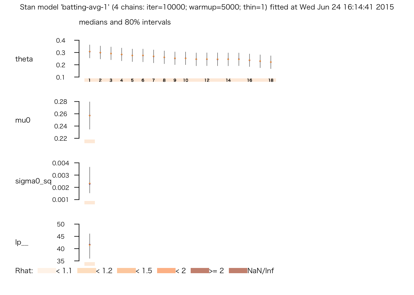
print(fit.2)## Inference for Stan model: batting-avg-1.
## 4 chains, each with iter=10000; warmup=5000; thin=1;
## post-warmup draws per chain=5000, total post-warmup draws=20000.
##
## mean se_mean sd 2.5% 25% 50% 75% 97.5% n_eff Rhat
## theta[1] 0.31 0.00 0.04 0.23 0.28 0.31 0.34 0.39 16528 1
## theta[2] 0.30 0.00 0.04 0.22 0.27 0.30 0.33 0.38 20000 1
## theta[3] 0.29 0.00 0.04 0.21 0.26 0.29 0.32 0.38 20000 1
## theta[4] 0.28 0.00 0.04 0.21 0.26 0.28 0.31 0.37 20000 1
## theta[5] 0.28 0.00 0.04 0.20 0.25 0.28 0.30 0.36 20000 1
## theta[6] 0.28 0.00 0.04 0.20 0.25 0.28 0.30 0.36 20000 1
## theta[7] 0.27 0.00 0.04 0.19 0.24 0.27 0.30 0.35 20000 1
## theta[8] 0.26 0.00 0.04 0.18 0.23 0.26 0.29 0.34 20000 1
## theta[9] 0.25 0.00 0.04 0.17 0.23 0.25 0.28 0.33 20000 1
## theta[10] 0.25 0.00 0.04 0.17 0.23 0.25 0.28 0.33 20000 1
## theta[11] 0.24 0.00 0.04 0.16 0.22 0.25 0.27 0.33 20000 1
## theta[12] 0.25 0.00 0.04 0.16 0.22 0.25 0.27 0.32 20000 1
## theta[13] 0.24 0.00 0.04 0.16 0.22 0.24 0.27 0.33 16353 1
## theta[14] 0.24 0.00 0.04 0.16 0.22 0.24 0.27 0.32 15329 1
## theta[15] 0.24 0.00 0.04 0.16 0.22 0.24 0.27 0.32 20000 1
## theta[16] 0.24 0.00 0.04 0.15 0.21 0.24 0.26 0.32 20000 1
## theta[17] 0.23 0.00 0.04 0.15 0.20 0.23 0.26 0.31 20000 1
## theta[18] 0.22 0.00 0.04 0.14 0.19 0.22 0.25 0.30 20000 1
## mu0 0.26 0.00 0.02 0.22 0.25 0.26 0.27 0.29 7878 1
## sigma0_sq 0.00 0.00 0.00 0.00 0.00 0.00 0.00 0.00 8046 1
## lp__ 41.24 0.06 3.97 32.47 38.78 41.59 44.12 47.86 4738 1
##
## Samples were drawn using NUTS(diag_e) at Wed Jun 24 16:14:41 2015.
## For each parameter, n_eff is a crude measure of effective sample size,
## and Rhat is the potential scale reduction factor on split chains (at
## convergence, Rhat=1).各打者の事後分布をヒストグラムで表す。
Post.theta <- extract(fit.2, "theta")$theta
Post.theta.df <- as.data.frame(Post.theta)
names(Post.theta.df) <- paste("theta", 1:18, sep = ".")
Post.theta.df <- Post.theta.df %>%
    gather(param, value, theta.1:theta.18)
theta.hist <- ggplot(Post.theta.df, aes(x = value, y = ..density..)) +
    geom_histogram() +
    facet_wrap( ~ param) +
    xlab("batting average")
print(theta.hist)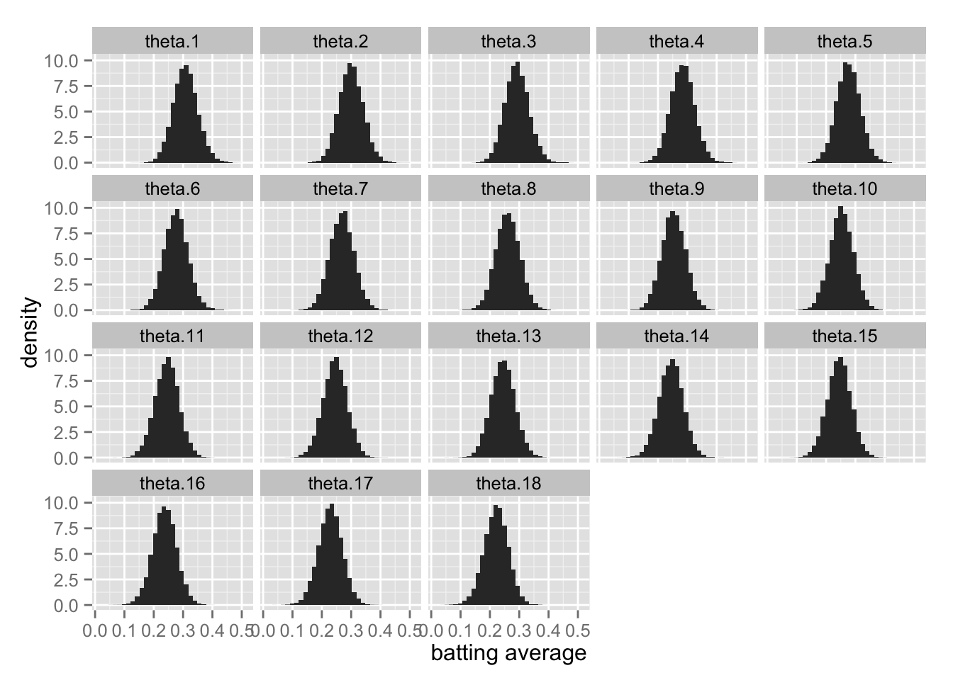
1-4, 1-5
省略
1-6
各モデルを推定して比較する代わりに、階層モデルの shrinkage を示す。
post.median <- apply(Post.theta, 2, median)
post.lower <- apply(Post.theta, 2, function(x) quantile(x, .025))
post.upper <- apply(Post.theta, 2, function(x) quantile(x, .975))
Post <- data.frame(average = EfronMorris$y,
                   med = post.median,
                   lower = post.lower,
                   upper = post.upper)
shrink <- ggplot(Post, aes(x = average, y = med)) +
    geom_linerange(aes(ymin = lower, ymax = upper), color = "tomato") +
    geom_point() +
    xlim(min(Post$lower), max(Post$upper)) +
    ylim(min(Post$lower), max(Post$upper)) +
    coord_fixed() +
    geom_abline(intercept = 0, slope = 1, color = "gray") +
    geom_hline(yintercept = mean(Post$average), color = "gray", linetype = "dashed")
shrink + labs(x = expression(paste("observed average, ", y[j])),
              y = expression(paste("95% posterior interval for ", theta[j])))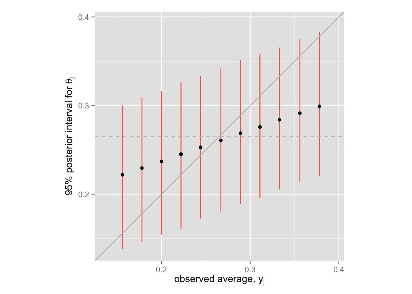
この図の中で、黒い点が \(\theta_j\) の事後分布の中央値、垂直に引かれた赤い線が \(\theta_j\) の95%事後区間である。 また、灰色の直線(45度線)が(ほぼ)separating の点推定値であり、灰色の点線が(ほぼ)pooling の点推定値である。階層モデル(partial pooling) によって、推定値がshrink していることが確認できる。
問2:打率の推定 二項分布モデル
与えられたモデルをStanモデルとして batting-avg-2.stan に書く。
// batting-avg-2.stan
data {
    int<lower=1> J;
    int<lower=0> r[J];
    int<lower=1> n[J];
}
parameters {
    real<lower=0, upper=1> theta[J];
    real<lower=0> alpha;
    real<lower=0> beta;
}
model {
    alpha ~ exponential(2);     // hyperprior
    beta ~ exponential(2);      // hyperprior
    theta ~ beta(alpha, beta);  // prior
    r ~ binomial(n, theta);     // likelihood
}
データをリストにする。
Bat.2 <- list(J = nrow(EfronMorris),
              r = EfronMorris$r,
              n = rep(45, nrow(EfronMorris)))
RStan で推定する。
fit.3 <- stan(file = "batting-avg-2.stan", data = Bat.2, iter = 1000, chains = 4)##
## TRANSLATING MODEL 'batting-avg-2' FROM Stan CODE TO C++ CODE NOW.
## COMPILING THE C++ CODE FOR MODEL 'batting-avg-2' NOW.
##
## SAMPLING FOR MODEL 'batting-avg-2' NOW (CHAIN 1).
##
## Iteration: 1 / 1000 [ 0%] (Warmup)
## Iteration: 100 / 1000 [ 10%] (Warmup)
## Iteration: 200 / 1000 [ 20%] (Warmup)
## Iteration: 300 / 1000 [ 30%] (Warmup)
## Iteration: 400 / 1000 [ 40%] (Warmup)
## Iteration: 500 / 1000 [ 50%] (Warmup)
## Iteration: 501 / 1000 [ 50%] (Sampling)
## Iteration: 600 / 1000 [ 60%] (Sampling)
## Iteration: 700 / 1000 [ 70%] (Sampling)
## Iteration: 800 / 1000 [ 80%] (Sampling)
## Iteration: 900 / 1000 [ 90%] (Sampling)
## Iteration: 1000 / 1000 [100%] (Sampling)
## # Elapsed Time: 0.051254 seconds (Warm-up)
## # 0.046567 seconds (Sampling)
## # 0.097821 seconds (Total)
##
##
## SAMPLING FOR MODEL 'batting-avg-2' NOW (CHAIN 2).
##
## Iteration: 1 / 1000 [ 0%] (Warmup)
## Iteration: 100 / 1000 [ 10%] (Warmup)
## Iteration: 200 / 1000 [ 20%] (Warmup)
## Iteration: 300 / 1000 [ 30%] (Warmup)
## Iteration: 400 / 1000 [ 40%] (Warmup)
## Iteration: 500 / 1000 [ 50%] (Warmup)
## Iteration: 501 / 1000 [ 50%] (Sampling)
## Iteration: 600 / 1000 [ 60%] (Sampling)
## Iteration: 700 / 1000 [ 70%] (Sampling)
## Iteration: 800 / 1000 [ 80%] (Sampling)
## Iteration: 900 / 1000 [ 90%] (Sampling)
## Iteration: 1000 / 1000 [100%] (Sampling)
## # Elapsed Time: 0.059676 seconds (Warm-up)
## # 0.03684 seconds (Sampling)
## # 0.096516 seconds (Total)
##
##
## SAMPLING FOR MODEL 'batting-avg-2' NOW (CHAIN 3).
##
## Iteration: 1 / 1000 [ 0%] (Warmup)
## Iteration: 100 / 1000 [ 10%] (Warmup)
## Iteration: 200 / 1000 [ 20%] (Warmup)
## Iteration: 300 / 1000 [ 30%] (Warmup)
## Iteration: 400 / 1000 [ 40%] (Warmup)
## Iteration: 500 / 1000 [ 50%] (Warmup)
## Iteration: 501 / 1000 [ 50%] (Sampling)
## Iteration: 600 / 1000 [ 60%] (Sampling)
## Iteration: 700 / 1000 [ 70%] (Sampling)
## Iteration: 800 / 1000 [ 80%] (Sampling)
## Iteration: 900 / 1000 [ 90%] (Sampling)
## Iteration: 1000 / 1000 [100%] (Sampling)
## # Elapsed Time: 0.057022 seconds (Warm-up)
## # 0.046262 seconds (Sampling)
## # 0.103284 seconds (Total)
##
##
## SAMPLING FOR MODEL 'batting-avg-2' NOW (CHAIN 4).
##
## Iteration: 1 / 1000 [ 0%] (Warmup)
## Iteration: 100 / 1000 [ 10%] (Warmup)
## Iteration: 200 / 1000 [ 20%] (Warmup)
## Iteration: 300 / 1000 [ 30%] (Warmup)
## Iteration: 400 / 1000 [ 40%] (Warmup)
## Iteration: 500 / 1000 [ 50%] (Warmup)
## Iteration: 501 / 1000 [ 50%] (Sampling)
## Iteration: 600 / 1000 [ 60%] (Sampling)
## Iteration: 700 / 1000 [ 70%] (Sampling)
## Iteration: 800 / 1000 [ 80%] (Sampling)
## Iteration: 900 / 1000 [ 90%] (Sampling)
## Iteration: 1000 / 1000 [100%] (Sampling)
## # Elapsed Time: 0.057607 seconds (Warm-up)
## # 0.042078 seconds (Sampling)
## # 0.099685 seconds (Total)fit.4 <- stan(fit = fit.3, data = Bat.2, iter = 10000, chains = 4)##
## SAMPLING FOR MODEL 'batting-avg-2' NOW (CHAIN 1).
##
## Iteration: 1 / 10000 [ 0%] (Warmup)
## Iteration: 1000 / 10000 [ 10%] (Warmup)
## Iteration: 2000 / 10000 [ 20%] (Warmup)
## Iteration: 3000 / 10000 [ 30%] (Warmup)
## Iteration: 4000 / 10000 [ 40%] (Warmup)
## Iteration: 5000 / 10000 [ 50%] (Warmup)
## Iteration: 5001 / 10000 [ 50%] (Sampling)
## Iteration: 6000 / 10000 [ 60%] (Sampling)
## Iteration: 7000 / 10000 [ 70%] (Sampling)
## Iteration: 8000 / 10000 [ 80%] (Sampling)
## Iteration: 9000 / 10000 [ 90%] (Sampling)
## Iteration: 10000 / 10000 [100%] (Sampling)
## # Elapsed Time: 0.492155 seconds (Warm-up)
## # 0.426203 seconds (Sampling)
## # 0.918358 seconds (Total)
##
##
## SAMPLING FOR MODEL 'batting-avg-2' NOW (CHAIN 2).
##
## Iteration: 1 / 10000 [ 0%] (Warmup)
## Iteration: 1000 / 10000 [ 10%] (Warmup)
## Iteration: 2000 / 10000 [ 20%] (Warmup)
## Iteration: 3000 / 10000 [ 30%] (Warmup)
## Iteration: 4000 / 10000 [ 40%] (Warmup)
## Iteration: 5000 / 10000 [ 50%] (Warmup)
## Iteration: 5001 / 10000 [ 50%] (Sampling)
## Iteration: 6000 / 10000 [ 60%] (Sampling)
## Iteration: 7000 / 10000 [ 70%] (Sampling)
## Iteration: 8000 / 10000 [ 80%] (Sampling)
## Iteration: 9000 / 10000 [ 90%] (Sampling)
## Iteration: 10000 / 10000 [100%] (Sampling)
## # Elapsed Time: 0.464371 seconds (Warm-up)
## # 0.395121 seconds (Sampling)
## # 0.859492 seconds (Total)
##
##
## SAMPLING FOR MODEL 'batting-avg-2' NOW (CHAIN 3).
##
## Iteration: 1 / 10000 [ 0%] (Warmup)
## Iteration: 1000 / 10000 [ 10%] (Warmup)
## Iteration: 2000 / 10000 [ 20%] (Warmup)
## Iteration: 3000 / 10000 [ 30%] (Warmup)
## Iteration: 4000 / 10000 [ 40%] (Warmup)
## Iteration: 5000 / 10000 [ 50%] (Warmup)
## Iteration: 5001 / 10000 [ 50%] (Sampling)
## Iteration: 6000 / 10000 [ 60%] (Sampling)
## Iteration: 7000 / 10000 [ 70%] (Sampling)
## Iteration: 8000 / 10000 [ 80%] (Sampling)
## Iteration: 9000 / 10000 [ 90%] (Sampling)
## Iteration: 10000 / 10000 [100%] (Sampling)
## # Elapsed Time: 0.440133 seconds (Warm-up)
## # 0.424998 seconds (Sampling)
## # 0.865131 seconds (Total)
##
##
## SAMPLING FOR MODEL 'batting-avg-2' NOW (CHAIN 4).
##
## Iteration: 1 / 10000 [ 0%] (Warmup)
## Iteration: 1000 / 10000 [ 10%] (Warmup)
## Iteration: 2000 / 10000 [ 20%] (Warmup)
## Iteration: 3000 / 10000 [ 30%] (Warmup)
## Iteration: 4000 / 10000 [ 40%] (Warmup)
## Iteration: 5000 / 10000 [ 50%] (Warmup)
## Iteration: 5001 / 10000 [ 50%] (Sampling)
## Iteration: 6000 / 10000 [ 60%] (Sampling)
## Iteration: 7000 / 10000 [ 70%] (Sampling)
## Iteration: 8000 / 10000 [ 80%] (Sampling)
## Iteration: 9000 / 10000 [ 90%] (Sampling)
## Iteration: 10000 / 10000 [100%] (Sampling)
## # Elapsed Time: 0.45428 seconds (Warm-up)
## # 0.409668 seconds (Sampling)
## # 0.863948 seconds (Total)plot(fit.4)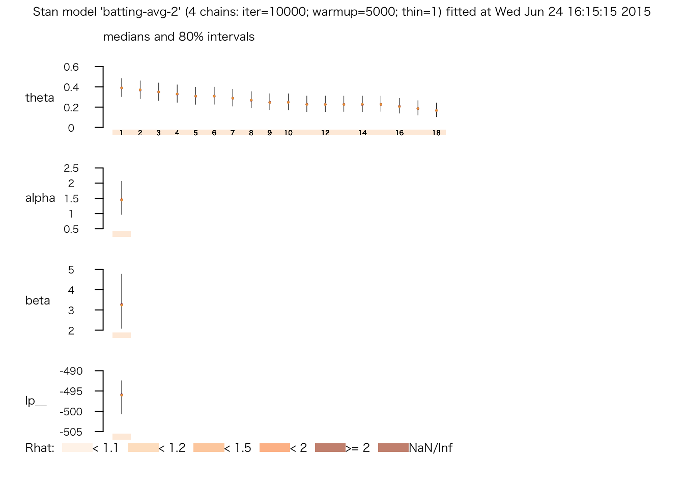
print(fit.4)## Inference for Stan model: batting-avg-2.
## 4 chains, each with iter=10000; warmup=5000; thin=1;
## post-warmup draws per chain=5000, total post-warmup draws=20000.
##
## mean se_mean sd 2.5% 25% 50% 75% 97.5%
## theta[1] 0.39 0.00 0.07 0.26 0.34 0.39 0.44 0.53
## theta[2] 0.37 0.00 0.07 0.24 0.32 0.37 0.42 0.51
## theta[3] 0.35 0.00 0.07 0.23 0.30 0.35 0.40 0.49
## theta[4] 0.33 0.00 0.07 0.21 0.28 0.33 0.38 0.47
## theta[5] 0.31 0.00 0.07 0.19 0.26 0.31 0.35 0.44
## theta[6] 0.31 0.00 0.07 0.19 0.27 0.31 0.35 0.45
## theta[7] 0.29 0.00 0.06 0.17 0.25 0.29 0.33 0.43
## theta[8] 0.27 0.00 0.06 0.16 0.23 0.27 0.31 0.40
## theta[9] 0.25 0.00 0.06 0.14 0.21 0.25 0.29 0.38
## theta[10] 0.25 0.00 0.06 0.14 0.21 0.25 0.29 0.38
## theta[11] 0.23 0.00 0.06 0.12 0.19 0.23 0.27 0.36
## theta[12] 0.23 0.00 0.06 0.12 0.19 0.23 0.27 0.36
## theta[13] 0.23 0.00 0.06 0.12 0.19 0.23 0.27 0.36
## theta[14] 0.23 0.00 0.06 0.12 0.19 0.23 0.27 0.36
## theta[15] 0.23 0.00 0.06 0.13 0.19 0.23 0.27 0.36
## theta[16] 0.21 0.00 0.06 0.11 0.17 0.21 0.25 0.33
## theta[17] 0.19 0.00 0.06 0.09 0.15 0.19 0.22 0.31
## theta[18] 0.17 0.00 0.05 0.08 0.13 0.17 0.20 0.29
## alpha 1.49 0.00 0.43 0.78 1.18 1.45 1.75 2.48
## beta 3.36 0.01 1.06 1.63 2.60 3.26 4.01 5.72
## lp__ -496.33 0.04 3.24 -503.55 -498.27 -495.98 -494.03 -491.04
## n_eff Rhat
## theta[1] 20000 1
## theta[2] 20000 1
## theta[3] 20000 1
## theta[4] 20000 1
## theta[5] 20000 1
## theta[6] 20000 1
## theta[7] 20000 1
## theta[8] 20000 1
## theta[9] 20000 1
## theta[10] 20000 1
## theta[11] 20000 1
## theta[12] 20000 1
## theta[13] 20000 1
## theta[14] 20000 1
## theta[15] 20000 1
## theta[16] 20000 1
## theta[17] 20000 1
## theta[18] 20000 1
## alpha 13575 1
## beta 13927 1
## lp__ 7755 1
##
## Samples were drawn using NUTS(diag_e) at Wed Jun 24 16:15:15 2015.
## For each parameter, n_eff is a crude measure of effective sample size,
## and Rhat is the potential scale reduction factor on split chains (at
## convergence, Rhat=1).各打者の事後分布をヒストグラムで表す。
Post.theta.2 <- extract(fit.4, "theta")$theta
Post.theta.df.2 <- as.data.frame(Post.theta.2)
names(Post.theta.df.2) <- paste("theta", 1:18, sep = ".")
Post.theta.df.2 <- Post.theta.df.2 %>%
    gather(param, value, theta.1:theta.18)
theta.hist <- ggplot(Post.theta.df.2, aes(x = value, y = ..density..)) +
    geom_histogram() +
    facet_wrap( ~ param) +
    xlab("batting average")
print(theta.hist)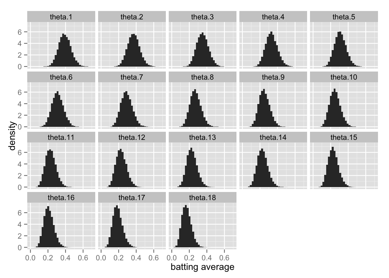
階層モデルの shrinkage を示す。
post.median <- apply(Post.theta.2, 2, median)
post.lower <- apply(Post.theta.2, 2, function(x) quantile(x, .025))
post.upper <- apply(Post.theta.2, 2, function(x) quantile(x, .975))
Post.2 <- data.frame(average = with(EfronMorris, r / 45),
                     med = post.median,
                     lower = post.lower,
                     upper = post.upper)
shrink <- ggplot(Post.2, aes(x = average, y = med)) +
    geom_linerange(aes(ymin = lower, ymax = upper), color = "tomato") +
    geom_point() +
    xlim(min(Post.2$lower), max(Post.2$upper)) +
    ylim(min(Post.2$lower), max(Post.2$upper)) +
    coord_fixed() +
    geom_abline(intercept = 0, slope = 1, color = "gray") +
    geom_hline(yintercept = mean(Post$average), color = "gray", linetype = "dashed")
shrink + labs(x = expression(paste("observed average, ", r[j] / 45)),
              y = expression(paste("95% posterior interval for ", theta[j])))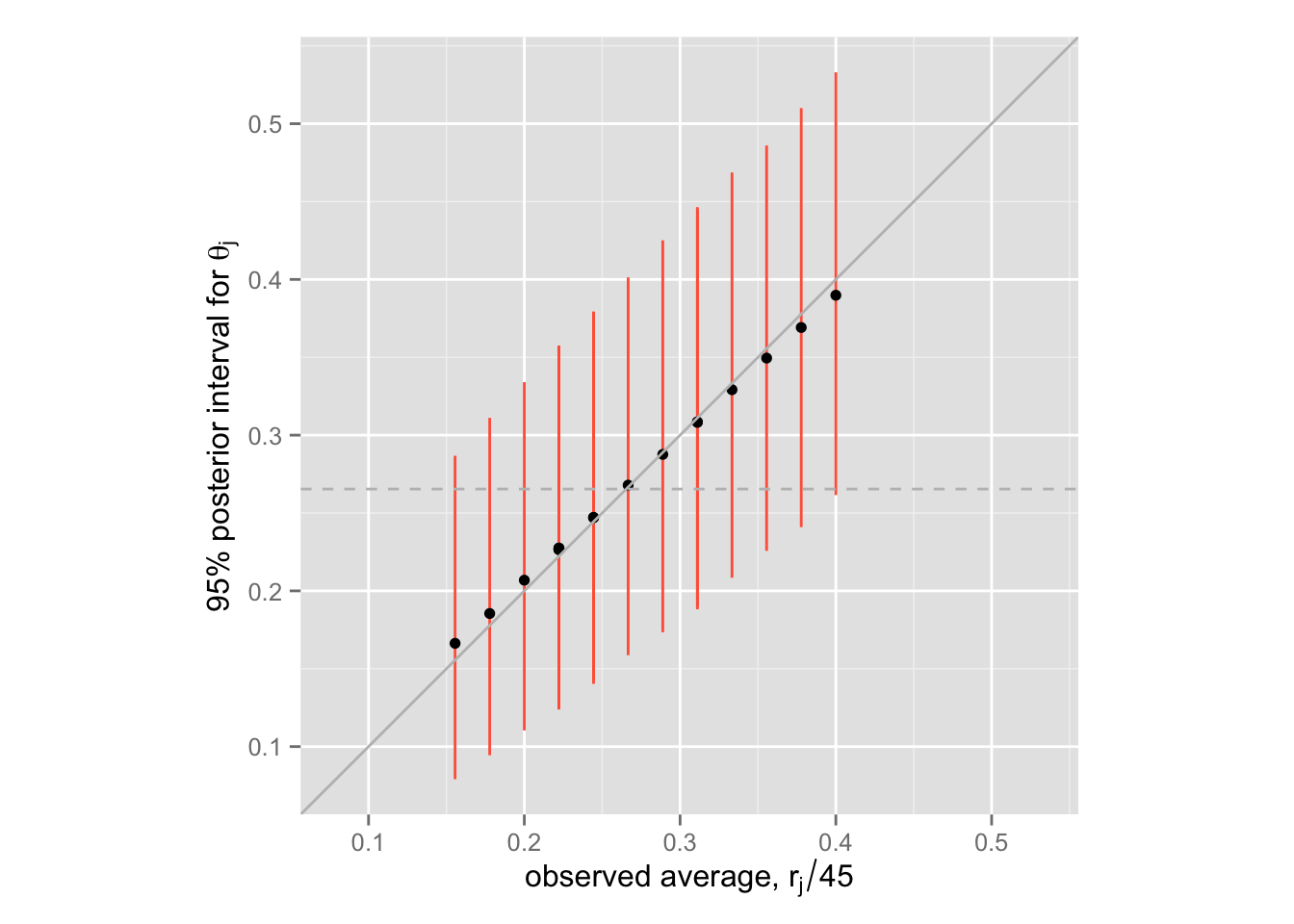
この図の中で、黒い点が \(\theta_j\) の事後分布の中央値、垂直に引かれた赤い線が \(\theta_j\) の95%事後区間である。 また、灰色の直線(45度線)が(ほぼ)separating の点推定値であり、灰色の点線が(ほぼ)pooling の点推定値である。階層モデル(partial pooling) によって、推定値がshrink していることが確認できる。
問1と比較すると、shrinkage が小さくなっていることがわかる。つまり、二項分布モデルのほうが、正規分布モデルのよりも separating に近い結果を出す。また、二項分布モデルの事後分布のほうがばらつきが大きいこともわかる。 これらの違いが生じる理由は?