Research Methods in Political Science I
Basic Statistics with R
Yuki Yanai
October 6, 2015
In this page, we will review basic statistics using R. Since expalanation given here is very brief, you are encouraged to consult the references listed on the course syllabus for more detailed review.
Summarizing Data
The first thing you should do in R is to set your working directory. The current working direcotry will be printed by typing
getwd()## [1] "/Users/yuki/Dropbox/teaching/kobe/rm1/2015/R"If you want to chage the working direcory, you can do so by setwd() function. For example, if you decided to use “methods” folder under your home directory as your working directory, type
setwd('~/methods/')“~/” is short for the home direcotry.
In RStudio, you should create/open a project rather than set the working directory. You can create a new project by choosing “File” -> “New Project”. RProject uses the project folder as the working directory, so you do not have to manually specify one.
Once you specify the working directory, all files you use for the project should be in that directory (or sub-directories of the working directory). Let’s save a data set fake-data-lec02.csv to your working directory.
Now let’s check if the data set exists in your working directory by typing dir() on Console. dir() prints the names of files in the directory. Confirming the data set is in your working directory, let’s load the data into R and name the data set “myd”. To read a csv file in R, we use read_csv() function in readr package (readr::read_csv()).
library("readr")
myd <- read_csv("fake-data-lec02.csv")
After you load a data set, you should always check the content of the data set. First, let’s display the first and the last 6 rows of the data set.
head(myd) ## the first 6 rows## id sex age height weight income
## 1 1 male 52 174.0 63.1 3475810
## 2 2 male 33 175.3 70.2 457018
## 3 3 male 22 175.0 82.6 1627793
## 4 4 male 33 170.1 81.8 6070642
## 5 5 male 26 167.4 51.2 1083052
## 6 6 male 37 159.3 57.8 2984929tail(myd) ## the last 6 rows## id sex age height weight income
## 95 95 female 21 165.4 56.3 1339138
## 96 96 female 65 161.1 46.8 6127136
## 97 97 female 45 161.2 48.7 1062663
## 98 98 female 53 166.2 64.2 10154200
## 99 99 female 43 158.1 48.5 8287163
## 100 100 female 48 153.8 42.0 1125390To check the variable names in the data set,
names(myd)## [1] "id" "sex" "age" "height" "weight" "income"To see how many observations and how many variables are in the data set,
dim(myd)## [1] 100 6The first number is \(n\) (the number of observations), and the second the number of columns or variables. In RStudio, these numbers are showin in “Environment” tab in the top right panel.
To examine the structure of the data set,
str(myd)## Classes 'tbl_df', 'tbl' and 'data.frame': 100 obs. of 6 variables:
## $ id : int 1 2 3 4 5 6 7 8 9 10 ...
## $ sex : chr "male" "male" "male" "male" ...
## $ age : int 52 33 22 33 26 37 50 30 62 51 ...
## $ height: num 174 175 175 170 167 ...
## $ weight: num 63.1 70.2 82.6 81.8 51.2 57.8 68.6 47.2 68.2 59.4 ...
## $ income: int 3475810 457018 1627793 6070642 1083052 2984929 1481061 1032478 1092943 3235943 ...To show summary statistics of the data set,
summary(myd)## id sex age height
## Min. : 1.00 Length:100 Min. :20.00 Min. :148.0
## 1st Qu.: 25.75 Class :character 1st Qu.:36.00 1st Qu.:158.1
## Median : 50.50 Mode :character Median :45.00 Median :162.9
## Mean : 50.50 Mean :45.96 Mean :163.7
## 3rd Qu.: 75.25 3rd Qu.:57.25 3rd Qu.:170.2
## Max. :100.00 Max. :70.00 Max. :180.5
## weight income
## Min. :28.30 Min. : 240184
## 1st Qu.:48.95 1st Qu.: 1343679
## Median :59.95 Median : 2987818
## Mean :59.18 Mean : 4343425
## 3rd Qu.:67.33 3rd Qu.: 6072696
## Max. :85.60 Max. :23505035Visualize Data
We use ggplot2 packages to make figures in R. To install the packages, type
install.packages("ggplot2", dependencies = TRUE, repos = "http://cran.ism.ac.jp")To load the package, type
library("ggplot2")
## To use Japanese characters, set font family as follows
# theme_set(theme_gray(base_size=12, base_family="HiraKakuProN-W3"))
We will learn to use ggplot2 in Week 4. Today, just copy and paste the codes to make figures, but try to make similar figures with other variables
Histograms
Let’s make a histogram of the variable height.
hist_height <- ggplot(myd, aes(height))
hist_height + geom_histogram()
## stat_bin: binwidth defaulted to range/30. Use 'binwidth = x' to adjust this.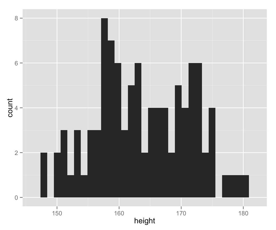
To save the figure created by ggpot(), we use ggsave() function. Fo instance,
ggsave('height-histogram.pdf')saves the last figure you made as “height-histogram.pdf” in the working directory. In RStudio, you can save the figure in the bottom right panel by clicking “Export” on top fo the figure.
You can also draw graphs without ggplot2.
hist(myd$height, xlab = "height", ylab = "count", main = "", col = "gray")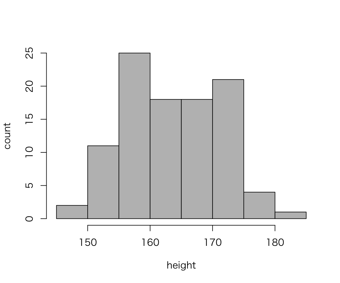
What are diffreces between the two histograms we created?
The vertical axis of histograms is row count (or frequency) by default. Let’s use density for the vertical axis, instead.
hist_height +
    geom_histogram(aes(y = ..density..))
## stat_bin: binwidth defaulted to range/30. Use 'binwidth = x' to adjust this.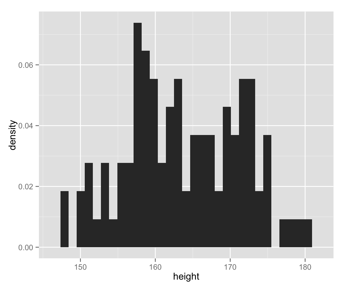
Without ggplot2,
hist(myd$height, probability = TRUE, col = "gray",
     xlab = "height", ylab = "density", main = "")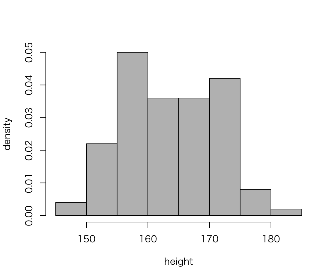
The bin width (or the number of classes) changes the apperance of histograms, and we should manually choose the best bin width. Let’s change the bin width to 5.
hist_height +
    geom_histogram(binwidth = 5)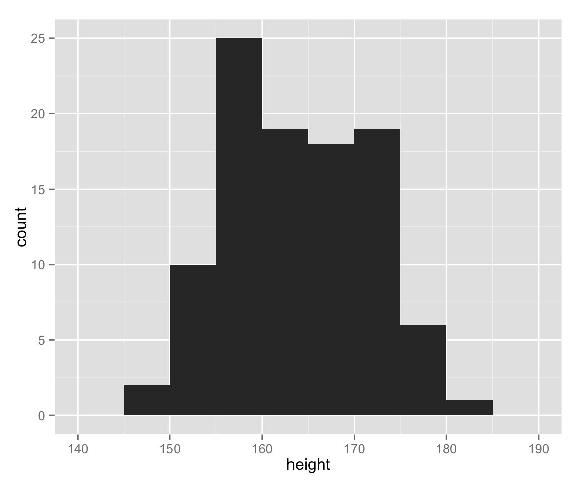
Now, the histogram drawn with ggplot2 looks very similar to one without.
So far, we have treated female and male together. Let’s draw a histogram for each gender.
hist_height +
    geom_histogram(binwidth = 5) +
    facet_wrap( ~ sex)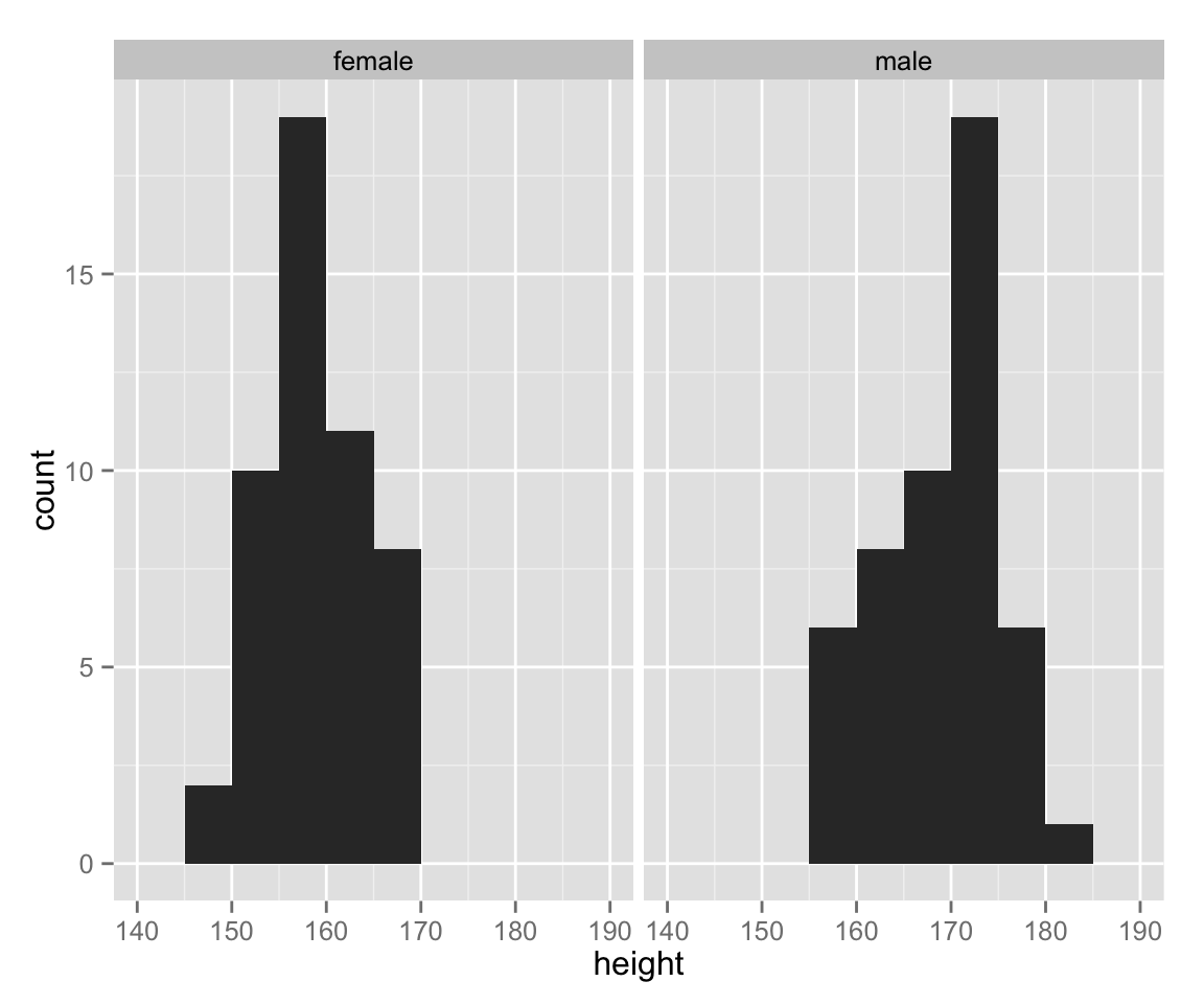
As we can see, the range of height differs between gender. Let’s use an appropriate range for each sex.
hist_height +
    geom_histogram(binwidth = 5) +
    facet_wrap( ~ sex, scales = "free_x")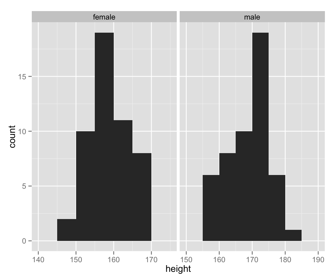
Box[-and Whisker] Plots
Next, let’s make box plots for female and male heights.
box_height <- ggplot(myd, aes(sex, height))
box_height + geom_boxplot() 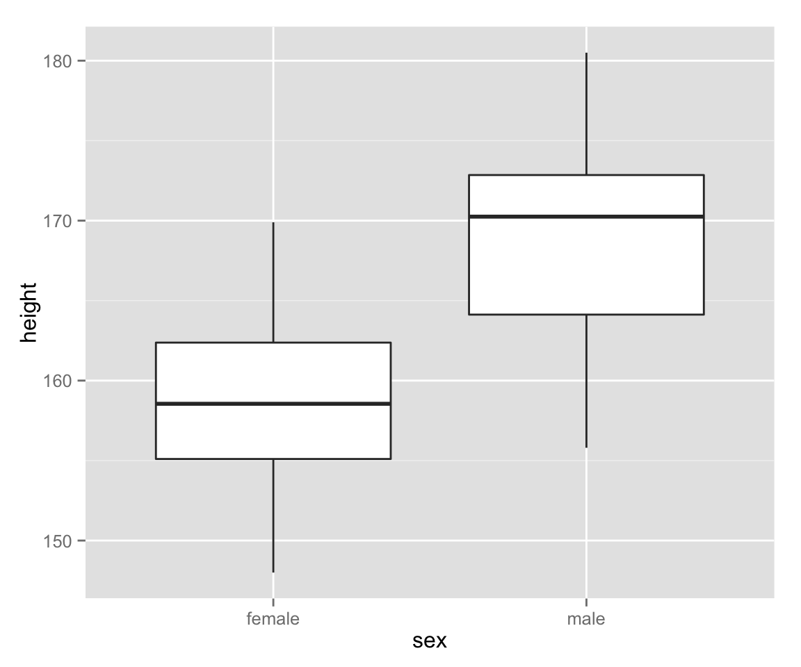
Scatter Plots
Now let’s examine the relationship between height and weight by a scatter plot.
scat_ht_wt <- ggplot(myd, aes(height, weight))
scat_ht_wt + geom_point()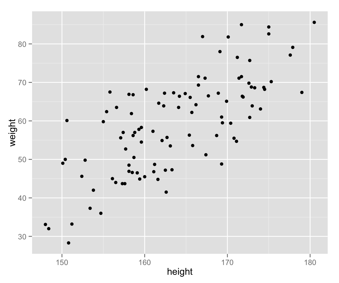
Use different colors for different genders.
scat_ht_wt + geom_point(aes(color = sex))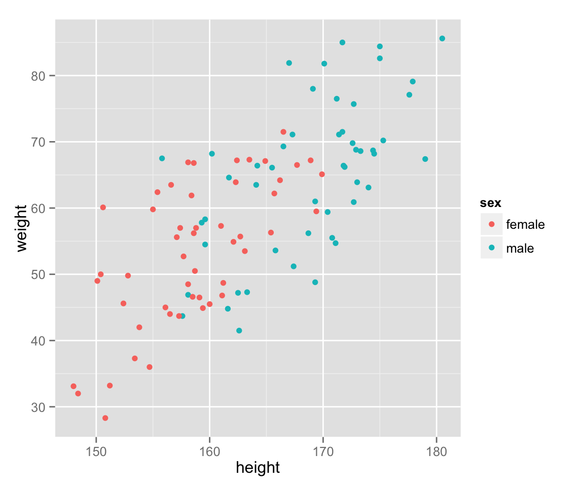
Add a (regression) line to show a relationship between the variables.
last_plot() + geom_smooth(method = 'lm', se = FALSE, aes(color = sex))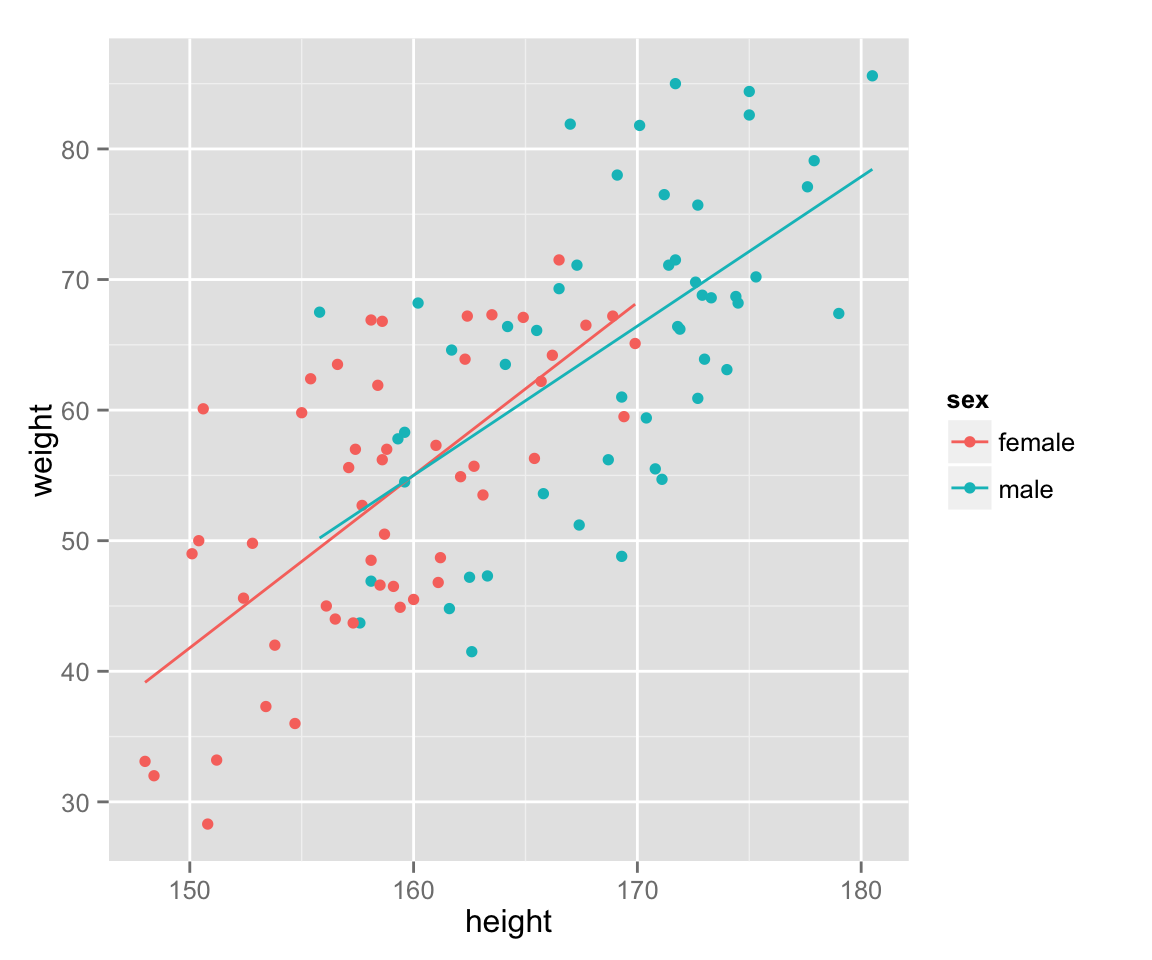
Lastly, add income to the graph.
scat_ht_wt + geom_point(aes(color = sex, size = income))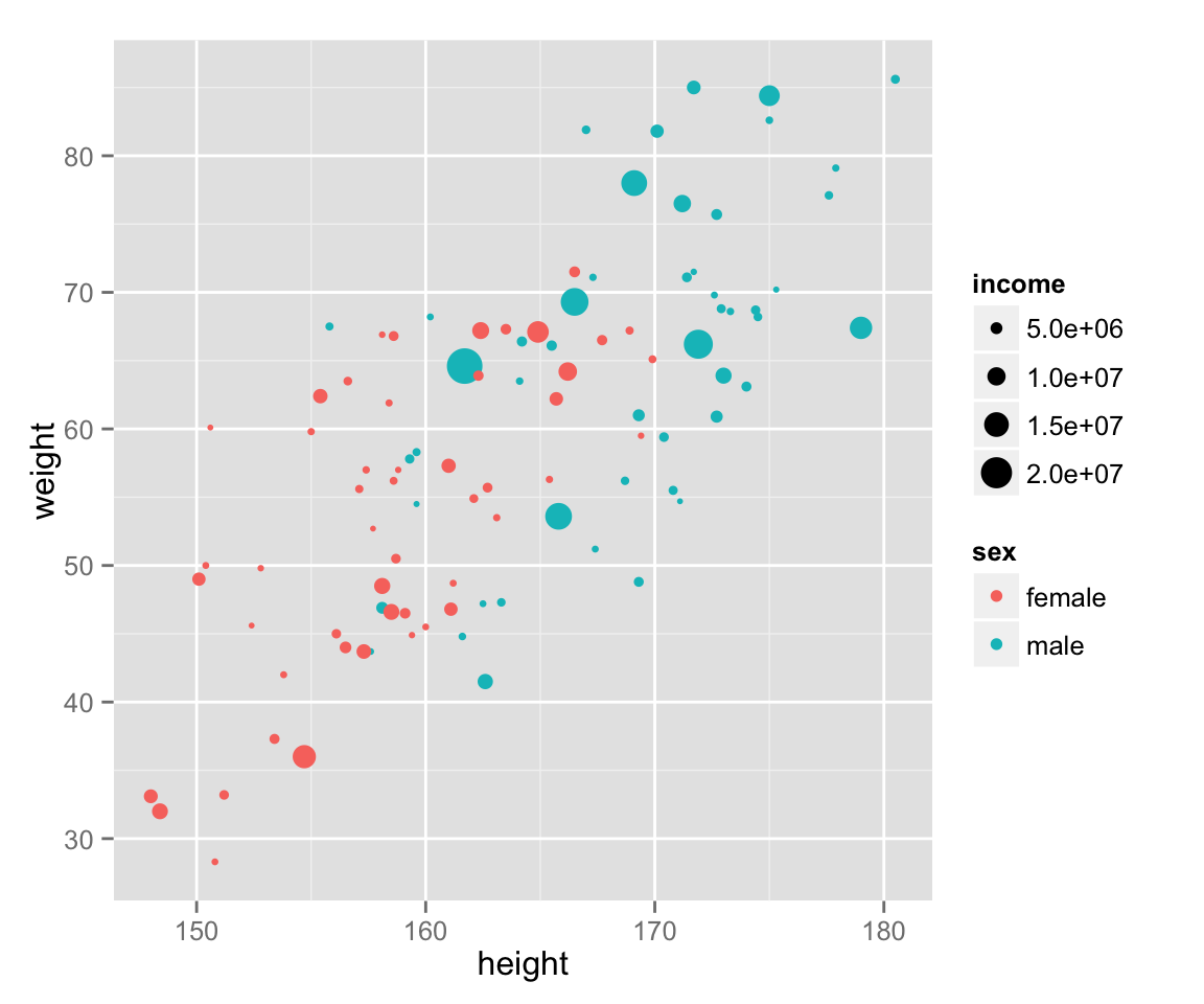
Statistics
Measures of Central Tendency
The mean of a variable \(x\) is denoted as \(\bar{x}\) (reads “x bar”): \[ \bar{x} = \frac{\sum_{i=1}^n x_i}{n}.\] In R, you can calculate the mean as follows.
x <- rnorm(20, mean = 10, sd = 4)  ## randomly draw 20 x's from N(10, 16)
sum(x) / length(x)
## [1] 10.28859Since you will calculate the mean over and over for a lot of different variables, you might want to have a function to get the means. In R, you can create your own functions. Let’s make a function to obtain the mean.
get_mean <- function(x) {
    return(sum(x) / length(x))
}
Now you can get the mean by the function get_mean().
get_mean(x)## [1] 10.28859However, such a basic function is built in. You can get the mean by mean() (how easy!).
mean(x)## [1] 10.28859Similarly, you can obtain the median, the minimum, and the maximum by median(), min(), and max(), respectively.
median(x)## [1] 10.64403min(x)## [1] 3.541893max(x)## [1] 14.40589Quantiles
You can calculate quantiles by quantile(). You also use this function to get percentiles or quartiles.
## 50% quantile = 50th percentile = median
quantile(x, 0.5)
## 50%
## 10.64403## 25th percentile = 1st quartile and 75th pecentile = 3rd quartile
quantile(x, c(.25, .75))## 25% 75%
## 8.739724 11.712385Thus, you get the inter-quartile range (IQR) as follows.
quantile(x, .75) - quantile(x, .25)## 75%
## 2.972662Alternatively, you can use
IQR(x)## [1] 2.972662The five number (0th to 4th quartiles) summary can be obtained by
quantile(x, c(0, .25, .5, .75, 1)) ## Five number summary with quartiles## 0% 25% 50% 75% 100%
## 3.541893 8.739724 10.644034 11.712385 14.405890If you would like to use hinges instead of the 1st and 3rd quartiles (See Tukey 1977. Exploratory Data Analysis.), use fivenum().
fivenum(x) ## Five number summary with hinges## [1] 3.541893 8.711931 10.644034 11.820155 14.405890Variance and Standard Deviation
The unbiased variance of a variance \(x\) is denoted as \(u_x^2\): \[u_x^2 = \frac{\sum_{i=1}^n (x_i - \bar{x})^2}{n-1}.\]
In R, you can calculate the variance as follows.
sum((x - mean(x))^2) / (length(x) - 1)## [1] 7.767437The variance is the most important statistic, and the function to get it is of course built in. You can get it by var().
var(x)## [1] 7.767437The standard deviation is the square root of the variance:
sqrt(var(x))## [1] 2.787012You can also use the built-in function sd().
sd(x)## [1] 2.787012Population Data
If the vector \(x\) is not a sample but the population, the mean and the variance of x are denoted as \(\mu\) and \(\sigma^2\), respectively. The mean of the population is obtained by the same function as the sample mean.
mean(x)## [1] 10.28859However, the formula for the population variance is different than the sample variance: \[\sigma^2 = \frac{\sum_{i=1}^N (x_i - \mu)^2}{N}.\] Therefore, you cannot use var(). Instead, you should write
var(x) * (length(x) - 1) / (length(x))## [1] 7.379065There is no built-in function for this. Let’s make a function.
pop_var <- function(x) {
    return(sum((x - mean(x))^2) / length(x))
}
pop_var(x)
## [1] 7.379065Probability Distributions
Random Draws from Probability Distributions
R has function to randomly draw numbers from some probability distributions.
For instance, you can draw \(n\) values from the continuous uniform distribution with the minimum \(a\) and the maximum \(b\) by runif(n, a, b) (“r” is for random, and “unif” for uniform). Let’s try with \(n = 10, a = 0, b = 1\):
runif(10, 0, 1)## [1] 0.56386205 0.40231370 0.76509556 0.65077447 0.26164666 0.58148090
## [7] 0.64719864 0.95906151 0.07985906 0.75215789Since this is a random draw, you will get a different set of numbers if you try again.
runif(10, 0, 1)## [1] 0.27511745 0.80627149 0.72606366 0.81551735 0.89329508 0.69382296
## [7] 0.40561214 0.59134272 0.04744498 0.06447589When we write papers or articles, we sometimes want the exactly same numbers again. In that case, we can set the seed of the random number by set.seed().
set.seed(2015-10-14)    ## set the seed
runif(10, 0, 1)
## [1] 0.15062308 0.23083080 0.01348260 0.53403895 0.79294008 0.66443619
## [7] 0.82853274 0.66335595 0.37601461 0.01377136set.seed(2015-10-14) ## use the same seed again
runif(10, 0, 1) ## can get the same values## [1] 0.15062308 0.23083080 0.01348260 0.53403895 0.79294008 0.66443619
## [7] 0.82853274 0.66335595 0.37601461 0.01377136You use a function rDISTRIBUTION_NAME() to draw numbers randomly from another distribution. For example, we use rnorm() for normal distributions, rt() for \(t\) distributions, and rchisq() for \(\chi^2\) distributions. However, you have to specify different sets of arguments (parameters) for different types of distributions. As already shown, you set the minimum and maximum for uniform distributions. For normal distributions, you specify the mean and standard deviation (sd). For \(t\) distributions and \(\chi^2\) distributions, the degree of freedom (df) must be given.
To randomly draw \(n\) values from N(\(\mu\), \(\sigma^2\)), for example, you write rnorm(n, mean = mu, sd = sigma). Let’s draw 100 values form the normal distribution with the man 10 and the variance 4.
x <- rnorm(100, 10, 2)You use the probability density function (PDF) \(f(x)\) by replacing “r” of rDISTRIBUTION-NAME() with “d” and the cumulative distribution function (CDF) \(F(x)\) with “p” (e.g, dnorm() and pnorm() for normal distributions).
Central Limit Theorem
The Central Limit Theorem (CLT) tells us that the sampling distribution of the sample mean is approximately normal with a large enough sample size \(n\), regardless of the distribution from which the sample is drawn. Thanks to CLT, we can make statistical inference about the large enough sample using the characteristics of noraml distributions. For example, we can use the fact that “95% of the values reside between \(\mu \pm 1.96 \sigma\) in a normal distribution” to infer that the 95% confidence interval is \([\bar{x} - 1.96\mathrm{SE}, \bar{x} + 1.96\mathrm{SE}]\) (SE stands for standard error, and it is the standard deviation of the sample means).
The central limit theorem is true, but it is little hard to understand why. Can we really approximate the distribution of the sample means by a normal distribution when the sample size is large enough? Let’s verify it with simulations!
Simulation 1: Sample Means of Discrete Uniform
There is a bag containing ten balls numbered 0 through 9. If you randomly choose a ball from the bag, there are ten possible numbers you get, and they are equally likely. Thus, the distribution of the number you get by drawing a ball is discrete uniform, and the mean of the possible values is 4.5.
Now, suppose that you do not know the numbers written on the balls. You will infer the true mean (popoulation mean) of the numbers by the sample mean. You will obtain the sample mean by drawing a ball \(n\) times from the bag. You will draw only a ball at a time, and put it back to the bag before you draw the next ball. That is, you conduct sampling with replacemnet. We will run a simulation to examine the sampling distribution obtained by this procedure.
First, make a bag contaning ten balls numbered 0 through 9.
bag <- 0:9Next, set the number of samples and the sample size (Note for Japanese speakers: 標本数と標本サイズの違いに注意).
trial <- 1000      ## the number of samples
n <- 1             ## sample size
Then, create a vector to save the simulation result. The length of the vector should match the number of samples. Before the simulation, we set each element to a missing value NA. (You can use any value to prepare a vector, but you should use NA because you can detect an error if the vector has NA after the simulation is run. If you use a numerical value, you cannot tell if it is the result of the simulation or the initial value.)
sample_means <- rep(NA, trial)Now let’s run the simulation. We draw a ball from the bag with the function sample(). To conduct smapling with replacement, we set the argument relace = TRUE. Every time we sample \(n\) values, we calculate the sample mean, and save it to the vector sample_means. We repeat this for each sample using for loop. R code:
for (i in 1:trial) {
    balls <- sample(bag, size = n, replace = TRUE)
    sample_means[i] <- mean(balls)
}
Now sample_means contains the simulation result. Let’s draw a histogram to see a sampling distribution (Note that this is merely a pseudo sampling distribution since the true sampling distribution must have every possible sample and usually only a theoretical distribution).
hist(sample_means, prob = TRUE, col = "gray", axes = FALSE,
     breaks = 0:10, right = FALSE,
     xlab = "sample mean", ylab = "",
     main = "Sampling distribution from Uniform: n = 1")
axis(1, 0.5:9.5, labels = 0:9)
abline(v = 5, col = "red", lwd = 2)  ## mark the population mean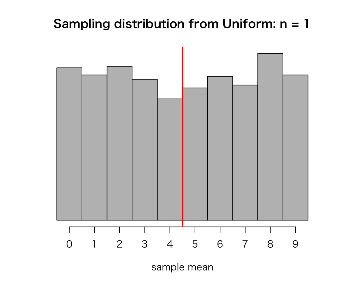
Does this look like normal? Probably not, because the sample size \(n\) is small (or not large enough). The histogram looks like the original uniform distribution, because \(n=1\).
What will happen as \(n\) gets larger? Run simulations! (See Assignment 2)