The t Test
Kobe Scientific IR/CP Seminar
Yuki Yanai
October 16, 2015
Preparation
In this page, we use 4 R packages. Please install them if necessary.
install.packages("ggplot2", dependencies = TRUE)
install.packages("haven", dependencies = TRUE)
install.packages("reshape2", dependencies = TRUE)
install.packages("dplyr", dependencies = TRUE)
The \(t\) Test
We use the \(t\) test to examine (1) if the mean of the sample is different than a specific value or (2) if the means of two groups are different. The \(t\) tests use Student’s \(t\) distribution, hence the name.
The central limit theorem assures that the error distribution is approximately normal if the sample size is large enough, but we sometimes have to deal with not-large-enough samples. William Sealy Gosset (aka “Student”) found that the errors follow \(t\) distribution with \(n-1\) degree of freedom even if the sample size \(n\) is not large enough. Therefore, we can use the characteristics of \(t\) distribution to make statistical inferences with small samples.
In the past, we use \(z\) test, which uses the standard normal distribution instead of \(t\), when \(n\) is large enough (say, \(n > 100\)) and use \(t\) test only for smaller samples. This is because it is tedious to prepare the large table of \(t\) distribution from which we find the critical value for the \(t\) test. However, since we can easily get the critical value using R (or Stata) instead of the table printed on paper, we don’t have to use \(z\) test anymore. The result of the \(t\) test converges to that of the \(z\) test as \(n\) gets large.
Why We Have to Test the Difference
We can caluculate the sample means. Therefore, the differnce is obvious in the samples. Then, why should we test the difference? To uderstand the reason, let’s make some fake data to examine. Here we suppose that people in the world evaluate Kobe University and Waseda University. These univerisity have the mean scores of 75 and 73, respectively, in the population. From this population, we sample 10 people and ask their evaluations. We would like to know if the evaluation differes between the two.
set.seed(12345)
kobe <- rnorm(10, mean = 75, sd = 3)    ## true mean evaluation is 75, with small sd
waseda <- rnorm(10, mean = 73, sd = 8)  ## true mean evaluation is 73, with large sd
df <- data.frame(kobe = kobe, waseda = waseda)
Now, let’s visualize the data we got.
library("ggplot2")
library("reshape2")
df_mlt <- melt(df) ## melt the data set into long format
## No id variables; using all as measure variablesuniv_box <- ggplot(df_mlt, aes(x = variable, y = value)) + geom_boxplot()
univ_box + labs(x = "university", y = "evaluation")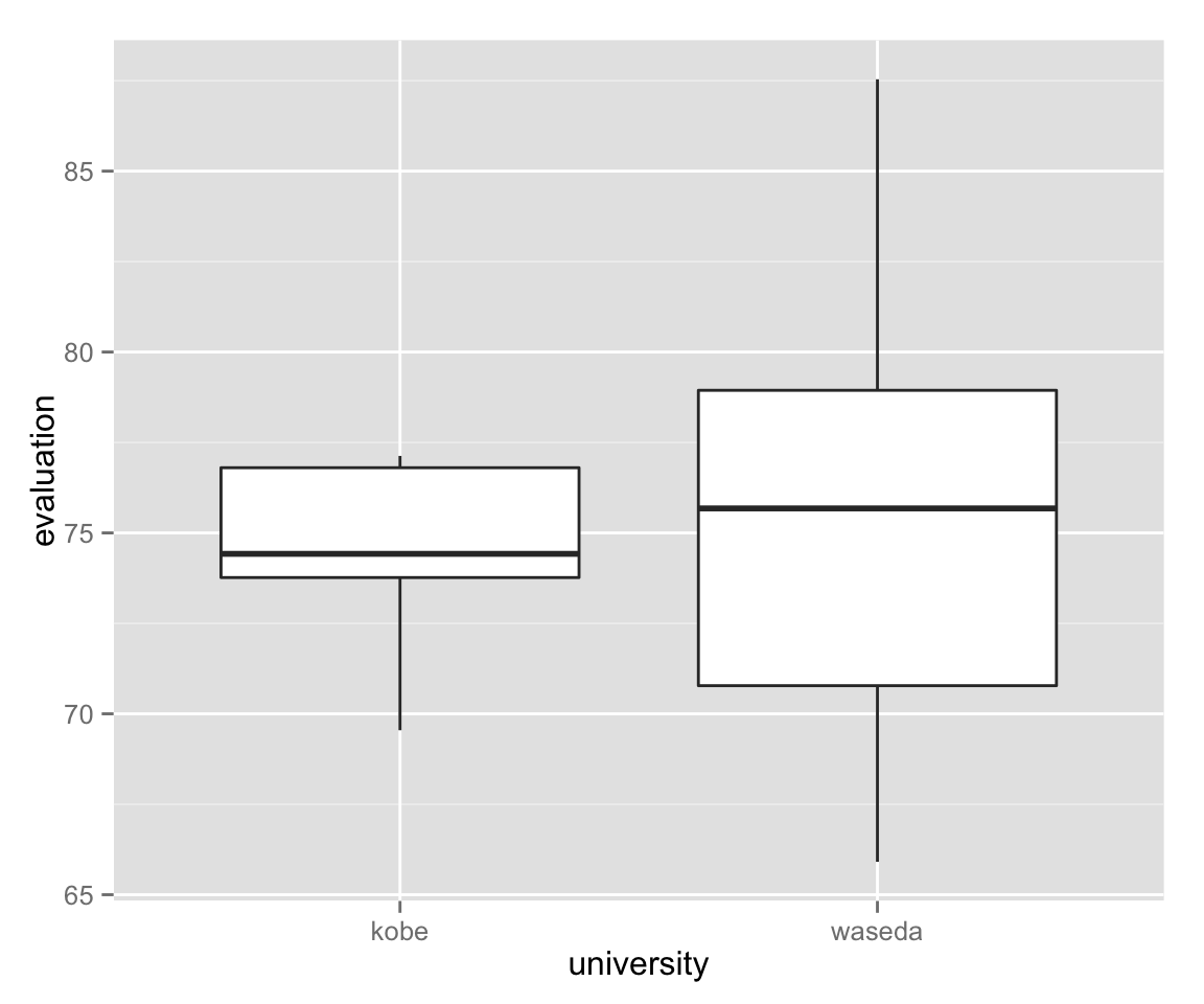
Let’s compare the summary statistics of the sample.
summary(df)## kobe waseda
## Min. :69.55 Min. :65.91
## 1st Qu.:73.77 1st Qu.:70.78
## Median :74.42 Median :75.68
## Mean :74.60 Mean :75.29
## 3rd Qu.:76.80 3rd Qu.:78.94
## Max. :77.13 Max. :87.54As we can see, Waseda university is slightly better evaluated than Kobe University in this sample. However, this is not what we want to know. We want to know if Waseda is thought better in the population (well, we actually know the answer: No). It can be the case that Waseda is better in this sample by chance. Therefore, we’d like to test if the difference is statistically significant or not.
In a typical \(t\) test, you should do the following.
- Define the null hypothesis, \(\mathrm{H_0}\).
- Define the alternative hypothesis, \(\mathrm{H_1}\)
- Calculate the test statistic.
- Find the critical values for the rejection region.
- Examine if the test statistic is in the rejection region.
- Conclude.
First, we have to set the null hypothesis. The null hypothesis is the hypothesis that we would like to reject to confiem our theory or predicition. It must point to a single value. Since we want to know if there is difference between two universities, let the null hypothesis be “no difference between two”: \[\mathrm{H}_0: d = d_0 = 0.\]
Next, define the alternative hypothesis. The null and alternative hypotheses must be mutually exclusive. Here, our alternative should be “there exists difference” or “difference is not zero”. \[\mathrm{H}_1: d \neq 0.\]
Then, we calculate the test statistic. Let \(x_i\) and \(y_i\) denote the scores given to the two universities by \(i\)th respondent. Then, we take the difference between two. \[d_i = x_i - y_i.\] The test statistic \(T\) is defined as \[T = \frac{\bar{d} - d_0}{\mathrm{sd}(d) / \sqrt{n}}.\] Simply put, this is similar to standardization of a normally distributed variable \(a\): \[z = \frac{a - \bar{a}}{\mathrm{sd}(a)}.\] Compare two formulae. For more detailed explanations, see Asano and Yanai(2013: ch.6, ch.7) or Freedman, Pisani, and Purves (2007: ch.26).
Now let’s calculate the test statistic \(T\).
x <- df$kobe
y <- df$waseda
d <- x - y
T <- (mean(d) - 0) / (sd(d) / sqrt(10))
T
## [1] -0.2797588Next, find the critical value(s) for the test. Since the sample size \(n = 10\), the test statitstic \(T\) would follow the \(t\) distribution with 9 degrees of freedom if the null hypothesis were true. To find the critical values, we have to set the significance level. Following the convention, let’s use 5 percent significance here. Because the critical values are 5 and 97.5 percentiles of the \(t\) distribtuion wiht df = 9, we can get them by qt() function in R.
qt(c(.025, .975), df = 9) ## get percentiles of t dist.## [1] -2.262157 2.262157The figure below shows the critical values and the significance level on \(t\) distribution. 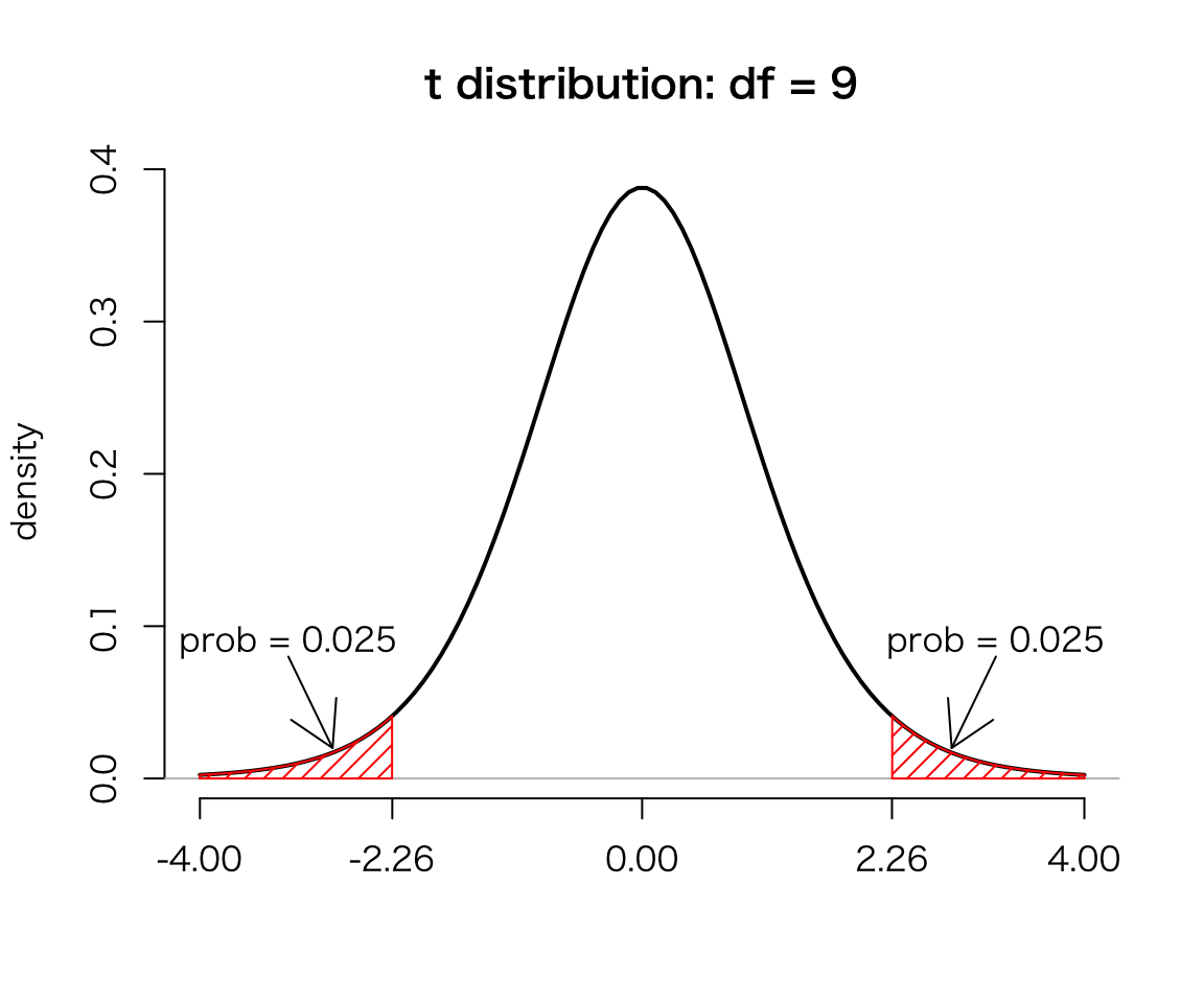
If \(T\) is inside the interval \([-2.26, 2.26]\), we cannot reject the null hypothesis. If it is outside the interval, we reject the null. Because the value of \(T\) is \(-0.28\), we can’t reject the null. Thus, we conclude that the difference between the two universities is not statistically significant.
Significance Level
What does it mean that the significance level is 5 percent? Well, it means that even if the null hypothesis is true, we wrongly reject the null 5 percent of the time. (Note for Japanese students: significance level should be called 有意水準(危険率). Never call it 有意確率. Unfortunately, some text books use 有意確率, but they shouldn’t because it is not the probability that something is significant.)
Let’s examine this by simulation.
Now, we take two samples with size 50 from the same population and compare the mean. Because the samples share the population, their means shouldn’t differ. However, we could (and usually do) get the different means in samples. When we conduct the \(t\) test for these samples, we would like to accept the null hypothesis of no difference. But theoretically, we wrongly reject the null 5 percent of the time.
The following function returns the rate of incorrect rejection of the null and shows the distribution of the test statistic \(T\).
sig_sim <- function(alpha = .05, n = 50, trials = 100) {
    ## Arguments:
    ##     alpha = significance level, default to 0.05
    ##     n = sample size, default to 50
    ##     trials = number of simulation trials, default to 100
    ## Return:
    ##     the rejection rate
    ## In addition, show the distribution of T

    ## vector to save the result
    res <- rep(NA, trials)
    T_vec <- rep(NA, trials)

    ## critical value
    cv <- abs(qt(alpha / 2, df = n -1))

    for (i in 1:trials) {
        x <- rnorm(50, mean = 50, sd = 5)
        y <- rnorm(50, mean = 50, sd = 5)
        d <- x - y
        T <- (mean(d) - 0) / (sd(d) / sqrt(n))
        T_vec[i] <- T
        res[i] <- abs(T) > cv
    }
    hist(T_vec, freq = FALSE, col = "gray",
         xlab = "test statistic",
         main = "Distribution of the test statistic")
    abline(v = c(-cv, cv), col = "red")
    return(mean(res))
}
sig_sim(trials = 10000)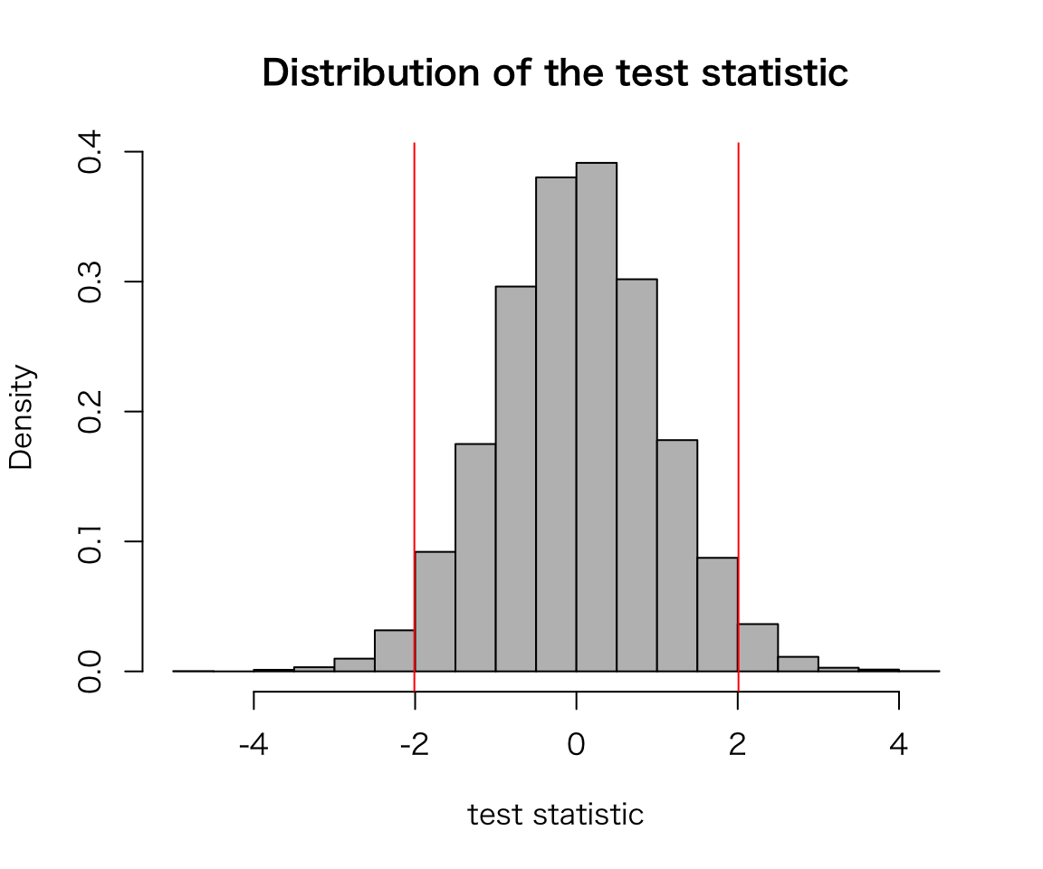
## [1] 0.0478As we can see, about 5 percent of the time, we get the wrong answer.
Let’s run the simulation with a different significance level, 10 percent.
sig_sim(alpha = .1, trials = 10000)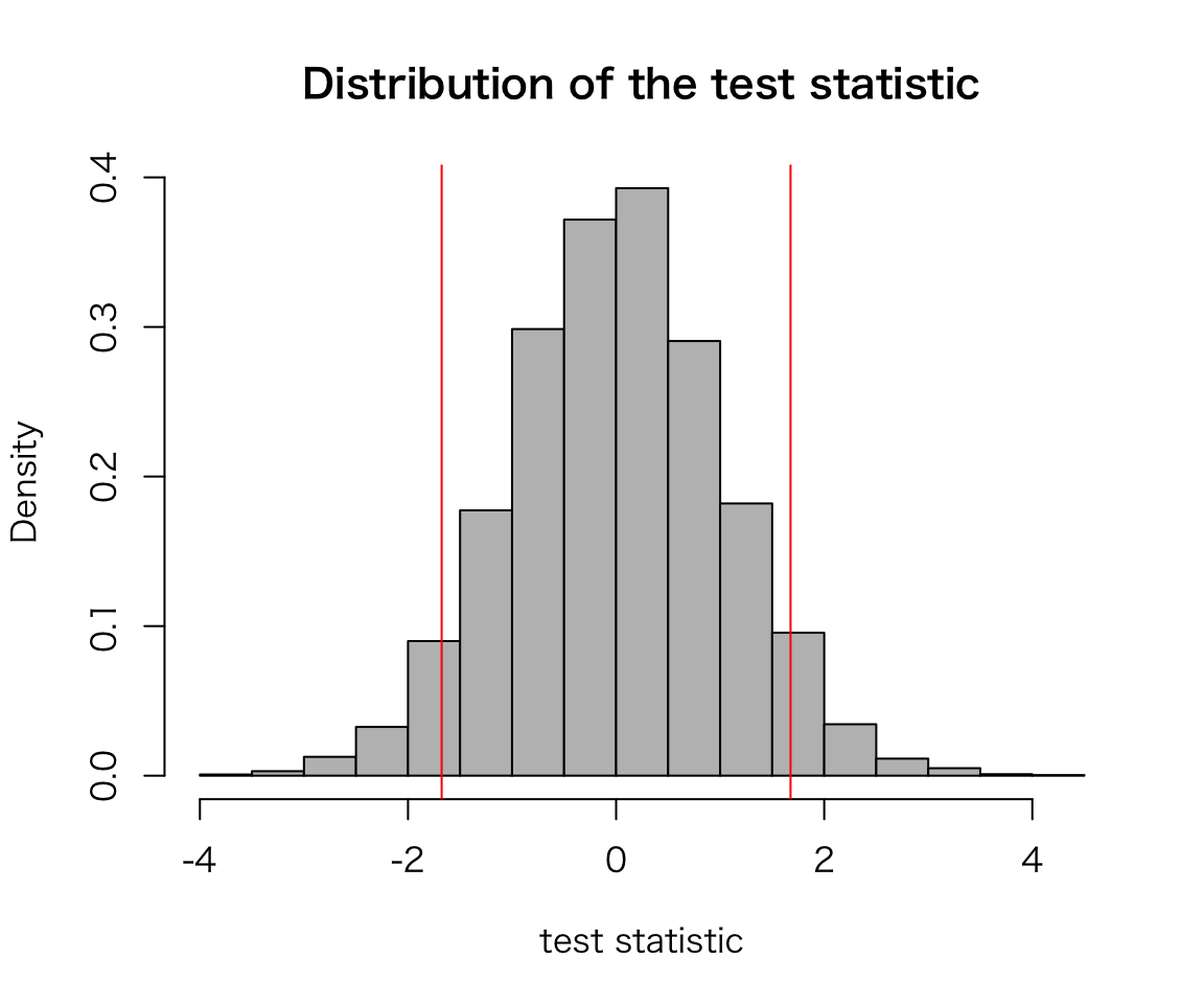
## [1] 0.1009Now the rate of wrong answers has increased to 10 percent.
Exercises
Ex. 1
Thirty people had dinner at a reastaurant. Let \(x_i\) denote the expense of the \(i\)-th person for the dinner. The mean of the expenses \(\bar{x} = 3,280\) yen and its standard deviaiton is 950 yen. Is the mean higher than 3,000 yen? Use the significance level of 5 percent (Ueda 2009: p.68).
Use R for the steps 3 through 5 above.
n <- 30
x_bar <- 3280
x_null <- 3000
x_sd <- 950
significance <- .05
## calculate the standard error
x_se <- x_sd / sqrt(n)
## calculate the test statistic
test_stat <- (x_bar - x_null) / x_se
## specify the rejection region in the t distribution
cv <- qt(significance / 2, df = n - 1)
## compare the test stat with the rejection region
abs(test_stat) > abs(cv)
## [1] FALSEEx. 2
A survey asked 30 students how much they spent on books in September this year (\(x\)) and last year (\(y\)). The mean of the difference (\(x - y\)) was 232 yen, and its standard deviation was 822 yen. Are two purchases different? Test it using 5 percent significance level (Ueda 2009: p.83).
n <- 30
dif_bar <- 232
dif_null <- 0
dif_sd <- 822
significance <- .05
## calculate the standard error
dif_se <- dif_sd / sqrt(n)
## calculate the test statistic
test_stat <- (dif_bar - dif_null) / dif_se
## specify the rejection region in the t distribution
cv <- qt(significance / 2, df = n - 1)
## compare the test stat with the rejection region
abs(test_stat) > abs(cv)
## [1] FALSEEx. 3
Masahiko Asano asked randomly chosen 10 students to taste ragular coffees of Starbucks and Tully’s. Each student evaluated each coffee using 0-100 scale. Test if the evaluation differs between two coffee companies with the 5 percent significan level (Asano and Yanai 2013: pp.139–146). The data set is available here in Stata format (.dta file). A Stata-format data set can be loaded into R by haven::read_dta() function.
library("haven")
myd <- read_dta("coffee_paired.dta")
First, let’s visualize the data.
myd_mlt <- melt(myd) ## melt the data set to long format## No id variables; using all as measure variablesbox_paired <- ggplot(myd_mlt, aes(x = variable, y = value)) + geom_boxplot()
box_paired + labs(x = "coffee shop", y = "evaluation")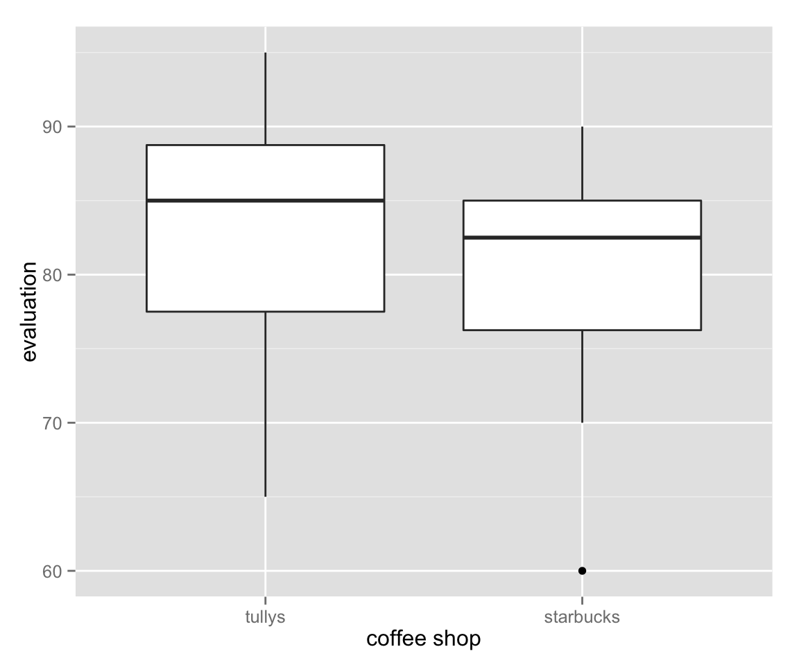
The figure tells us that Tully’s is slightly better than Starbucks, but not much.
Now, let’s test by manually calculating the test statistic.
n <- nrow(myd)
dif <- with(myd, tullys - starbucks)
dif_bar <- mean(dif)
dif_null <- 0
dif_sd <- sd(dif)
significance <- .05
## calculate the standard error
dif_se <- dif_sd / sqrt(n)
## calculate the test statistic
test_stat <- (dif_bar - dif_null) / dif_se
## specify the rejection region in the t distribution
cv <- qt(significance / 2, df = n - 1)
## compare the test stat with the rejection region
abs(test_stat) > abs(cv)
## [1] TRUEUnlike Ex. 1 or Ex. 2, here we have raw data (the values for each respondent). Thus, we can use R’s t.test() function to conduct the \(t\) test. Since our data is paired (meaning that both Tully’s and Starbuck’s coffees are tasted by the same students), we set the paired argument to TRUE.
t.test(myd$tullys, myd$starbucks, paired = TRUE)##
## Paired t-test
##
## data: myd$tullys and myd$starbucks
## t = 2.4495, df = 9, p-value = 0.03679
## alternative hypothesis: true difference in means is not equal to 0
## 95 percent confidence interval:
## 0.3059128 7.6940872
## sample estimates:
## mean of the differences
## 4Did we get the same results?
Ex. 4
Asano randomly sampled other 20 students. He asked 10 of them to drink Tully’s regular coffee and the other 10 to drink Starbuks’ regular coffee. Each sudent evaluated the coffee they had using 0-100 scale. Test if the evaluation differs between two gropus with the 5 percent significance level (Asano and Yanai 2013: pp.139–146). The data set is available here in Stata format (.dta file).
myd2 <- read_dta("coffee_unpaired.dta")
myd2
## score starbucks
## 1 95 0
## 2 95 0
## 3 85 0
## 4 90 0
## 5 85 0
## 6 75 0
## 7 85 0
## 8 85 0
## 9 75 0
## 10 65 0
## 11 90 1
## 12 85 1
## 13 85 1
## 14 80 1
## 15 85 1
## 16 70 1
## 17 85 1
## 18 75 1
## 19 80 1
## 20 60 1library("dplyr")##
## Attaching package: 'dplyr'
##
## The following objects are masked from 'package:stats':
##
## filter, lag
##
## The following objects are masked from 'package:base':
##
## intersect, setdiff, setequal, unionmyd2 <- myd2 %>%
mutate(starbucks = factor(starbucks, labels = c("Tully's", "Starbucks")))Visualize!
box_unpaired <- ggplot(myd2, aes(x = starbucks, y = score)) + geom_boxplot()
box_unpaired + xlab("coffee shop")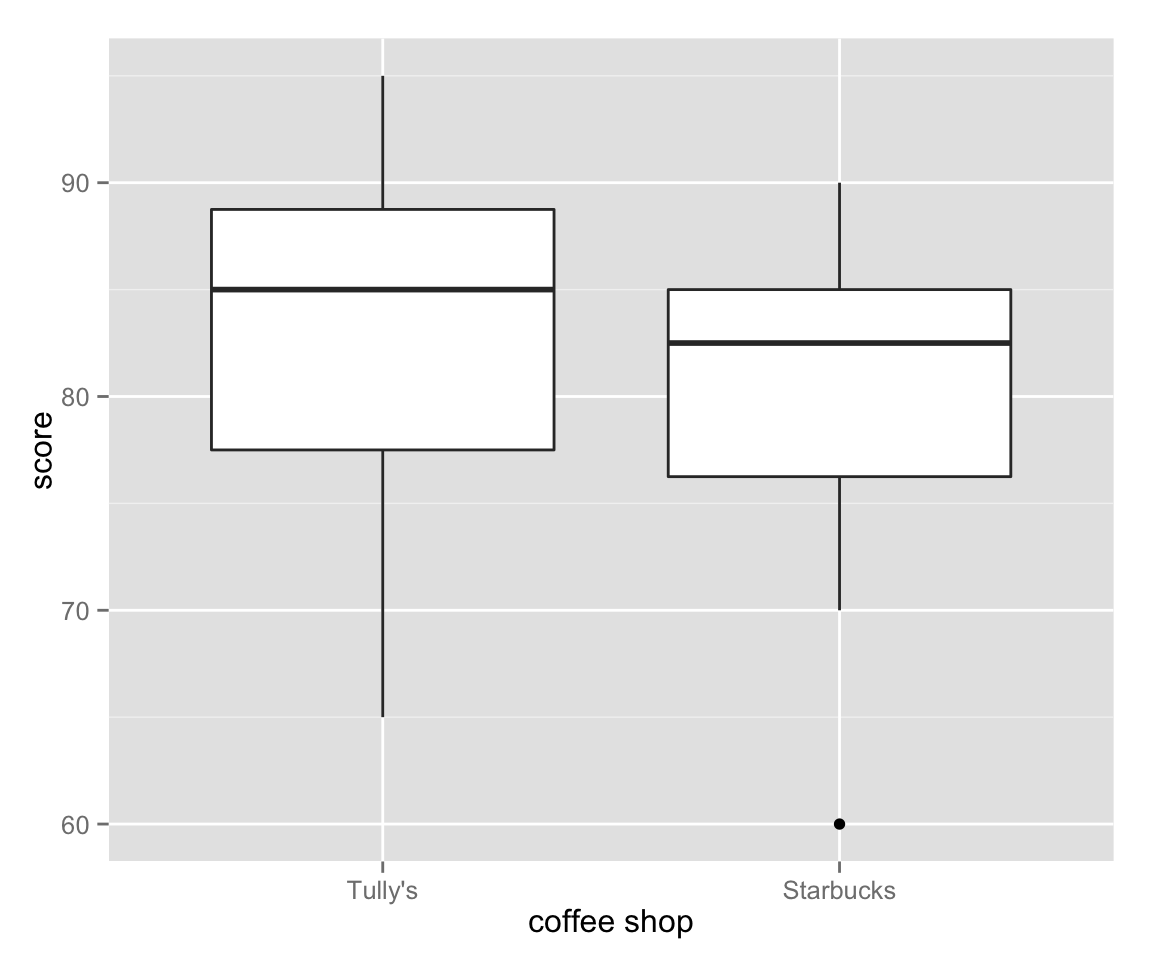
Again, Tully’s is slightly better than Starbucks, but not much.
Now, let’s test if the difference is statistically significant at 5 percent level. Since the data is unpaired (different coffees are tasted by different groups of the students), we set the paired argument to FALSE (In fact, you don’t have to specify it because it’s default to FALSE). By so doing, we conduct Welch’s \(t\) test.
t.test(score ~ starbucks, data = myd2)##
## Welch Two Sample t-test
##
## data: score by starbucks
## t = 0.97173, df = 17.951, p-value = 0.3441
## alternative hypothesis: true difference in means is not equal to 0
## 95 percent confidence interval:
## -4.649864 12.649864
## sample estimates:
## mean in group Tully's mean in group Starbucks
## 83.5 79.5
References
- Asano and Yanai (2013): 浅野正彦, 矢内勇生.『Stataによる計量政治学』オーム社.
- Freedman, David, Robert Pisani, and Roger Purves. (2007) Statistics, 4th ed. New York: W.W. Norton.
- Ueda (2009): 上田拓治.『44の例題で学ぶ統計的検定と推定の解き方』オーム社.