An Introduction to rgamer

Examples for useR! 2026 in Warsaw

Author

Yuki Yanai (w/ Yoshio Kamijo)

Published

June 4, 2026

Preparation

Install rgamer (if necessary).

#install.packages("pak")
pak::pak("yukiyanai/rgamer")

Load rgamer.

library(rgamer)

Normal-form games

Example 1: Prisoners’ dilemma (Not shown in the poster)

Define a normal-form game with normal_form().

game1 <- normal_form(
  players = c("Kamijo", "Yanai"),
  s1 = c("Stays silent", "Betrays"), 
  s2 = c("Stays silent", "Betrays"), 
  payoffs1 = c(-1,  0, -3, -2), 
  payoffs2 = c(-1, -3,  0, -2))

Find solutions of the game using solve_nfg().

sol_g1 <- solve_nfg(game1)

Pure-strategy NE: [Betrays, Betrays]

		Yanai
	strategy	Stays silent	Betrays
Kamijo	Stays silent	-1, -1	-3, 0^
	Betrays	0^, -3	-2^, -2^

Example 2: Stag hunt

Define a normal-form game with normal_form()

game2 <- normal_form(
  players = c("Kamijo", "Yanai"),
  s1 = c("Stag", "Hare"), 
  s2 = c("Stag", "Hare"), 
  payoffs1 = c(10, 8, 0, 7), 
  payoffs2 = c(10, 0, 8, 7))

Find solutions including mixed-strategy Nash equilibria using solve_nfg() with mixed = TRUE.

sol_g2 <- solve_nfg(game2, mixed = TRUE)

Pure-strategy NE: [Stag, Stag], [Hare, Hare]

Mixed-strategy NE: [(7/9, 2/9), (7/9, 2/9)]

The obtained mixed-strategy NE might be only a part of the solutions.

Please examine br_plot (best response plot) carefully.

		Yanai
	strategy	Stag	Hare
Kamijo	Stag	10^, 10^	0, 8
	Hare	8, 0	7^, 7^

Examine the best-response plot (br_plot)

sol_g2$br_plot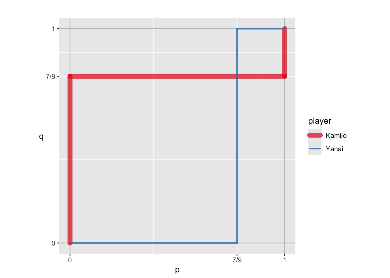

The plot shows that there are three intersections of the two correspondences: two pure-strategy NEs, (Stag, Stag) and (Hare, Hare), and a mixed-strategy NE, ((7/9, 2/9), (7/9, 2/9)).

Example 3: Cournot competition

Define a game of which payoffs are given by functions.

game3 <- normal_form(
  players = c("Firm 1", "Firm 2"),
  pars = c("x1", "x2"),
  par1_lim = c(0, 30),
  par2_lim = c(0, 30),
  payoffs1 = "x1 * (20 - x1 - x2)",
  payoffs2 = "x2 * (16 - x1 - x2)"
)

Find solutions of the game.

sol_g3 <- solve_nfg(game3, plot = FALSE)

approximated NE: (8, 4)

The obtained NE might be only a part of the solutions.
Please examine br_plot (best response plot) carefully.

Show the best-response plot with NE marked.

sol_g3$br_plot_NE

Extensive-form games

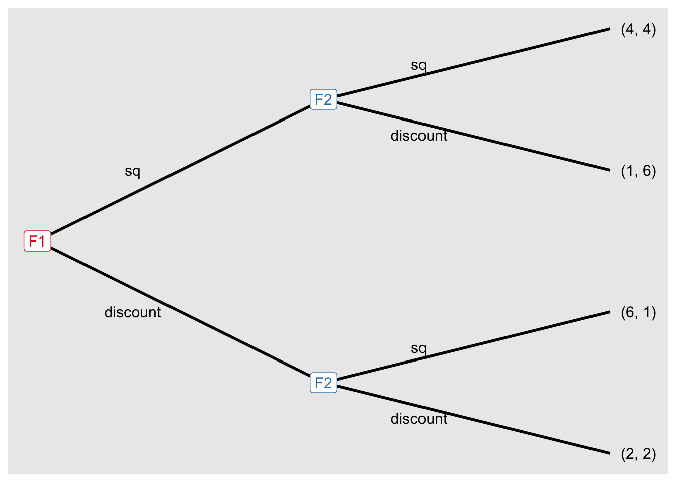
Example 4: Price competition

Define an extensive-form game with extensive_form().

game4 <- extensive_form(
  players = list("F1", 
                 rep("F2", 2),
                 rep(NA, 4)),
  actions = list(c("sq", "discount"),
                 c("sq", "discount"), c("sq", "discount")),
  payoffs = list(F1 = c(4, 1, 6, 2),
                 F2 = c(4, 6, 1, 2)),
  show_node_id = FALSE,
  direction = "right"
)

Find solutions of the game by backward induction using solve_efg().

sol_g4 <- solve_efg(game4)

backward induction: [(discount), (discount, discount)]

Show the tree.

sol_g4$trees[[1]]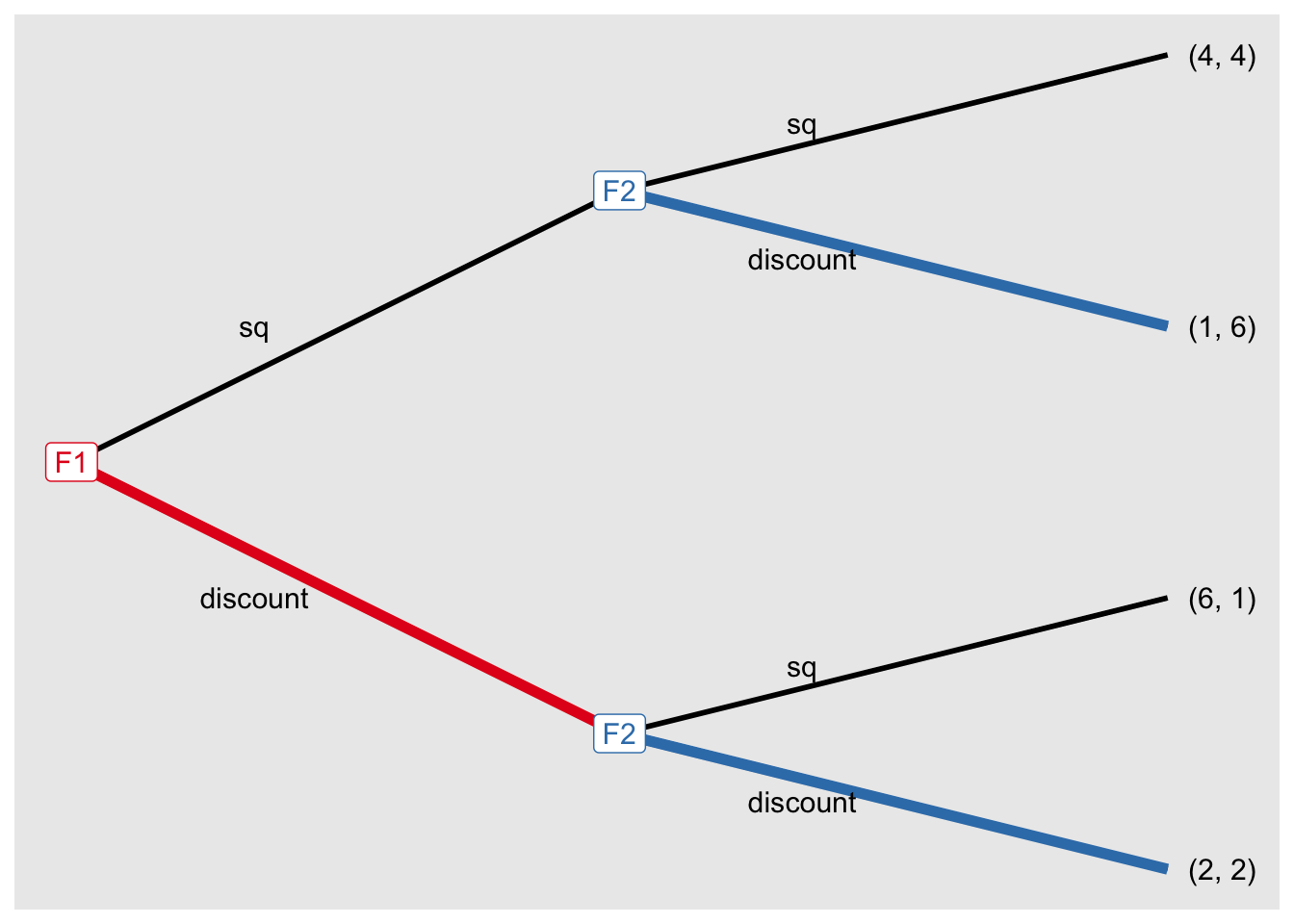

Two-player extensive-form games can be transformed into a normal-form game by to_matrix()

g4nf <- to_matrix(game4)

Since g4nf is a normal-form game, you can find NEs using solve_nfg().

sol_g4nf <- solve_nfg(g4nf)

Pure-strategy NE: [(discount), (discount, discount)]

		F2
	strategy	(sq, sq)	(sq, discount)	(discount, sq)	(discount, discount)
F1	(sq)	4, 4	4^, 4	1, 6^	1, 6^
	(discount)	6^, 1	2, 2^	6^, 1	2^, 2^

Example 5: Ultimatum game with the entrance stage

Define an extensive-form game of imperfect information with extensive_form(), where you must specify info_set.

game5 <- extensive_form(
  players = list("P",
                 c("P", NA),
                 rep("R", 2),
                 rep(NA, 4)),
  actions = list(c("join", "not join"),
                 c("8:2", "5:5"),
                 c("accept", "rejct"),
                 c("accept", "rejct")),
  payoffs = list(P = c(3, 8, 0, 5, 0),
                 R = c(3, 2, 0, 5, 0)),
  info_sets = list(c(4, 5)),
  direction = "right",
  show_node_id = FALSE
)

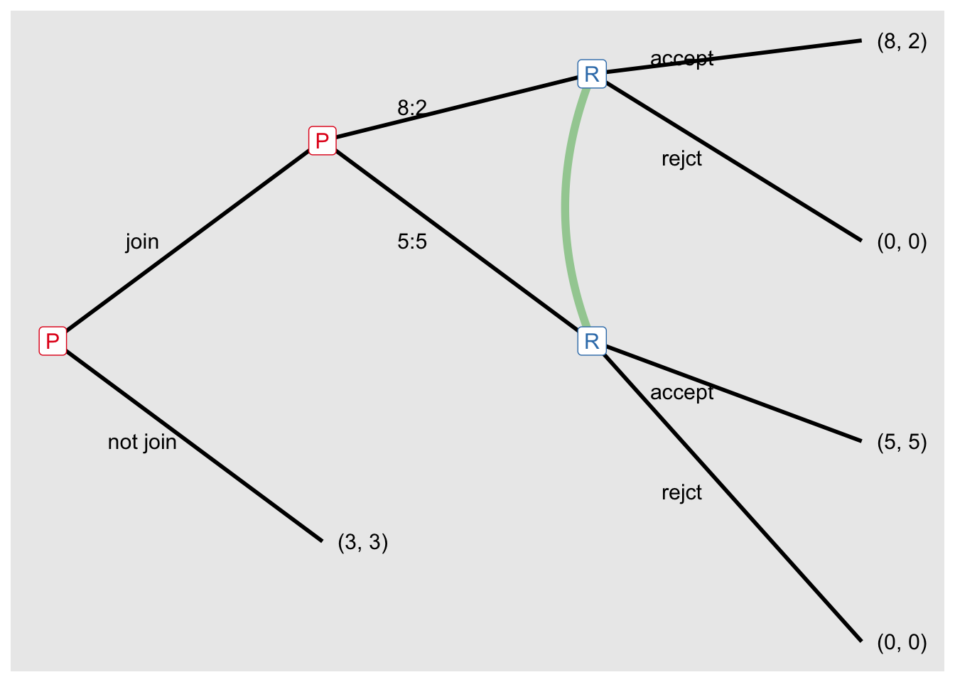
Find sub-game perfect equilibria with solve_eft() with concept = "spe".

sol_g5 <- solve_efg(game5, concept = "spe")

SPE: [(join, 8:2), (accept)]

Show the tree

sol_g5$tree

[[1]]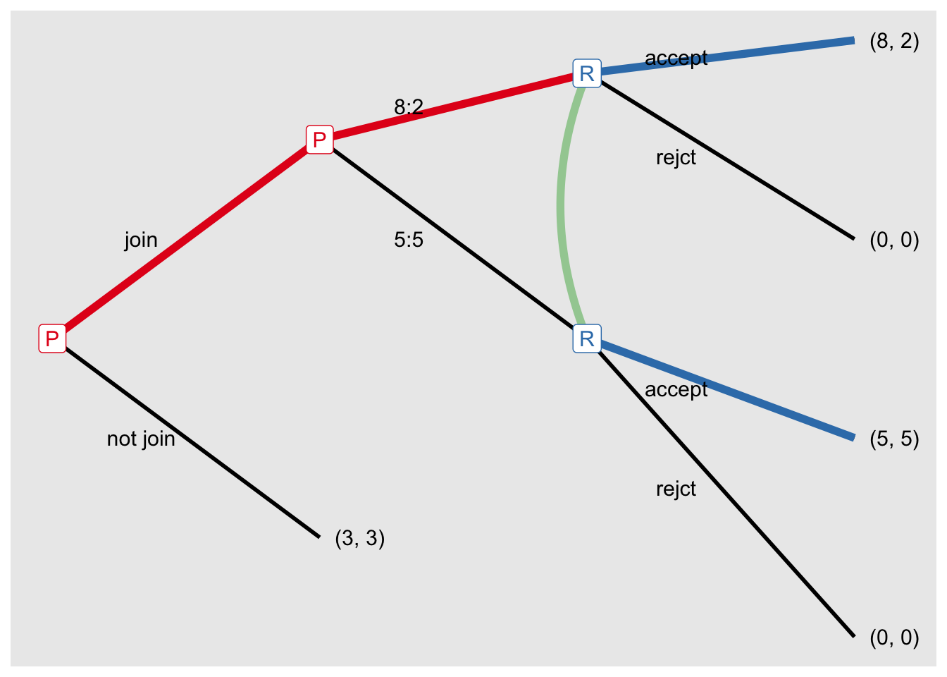

Simulating learning processes

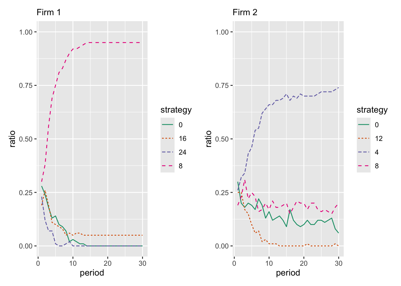
Example 6: Reinforcement learning in Cournot competition

Define a Cournot competition with discretized payoffs.

game6 <- normal_form(
  players = c("Firm 1", "Firm 2"),
  pars = c("x1", "x2"),
  par1_lim = c(0, 24),
  par2_lim = c(0, 12),
  payoffs1 = "(20 - x1 - x2) * x1",
  payoffs2 = "(16 - x1 - x2) * x2",
  discretize = TRUE,
  discrete_points = c(4, 4)
)

Simulate reinforcement learning with sim_learning() with type = "reinforcement".

set.seed(2026-06-04)

g6_reinf <- sim_learning(game6,
                         n_samples = 100,
                         n_periods = 30,
                         type = "reinforcement",
                         lambda = 0.1,
                         plot_range_y = c(0, 1))

Show the results.

g6_reinf$plot_mean