Overview
The goal of rgamer is to help students learn Game Theory using R. The functions prepared by the package not only solve basic games such as two-person normal-form games but also provide the users with visual displays that highlight some aspects of the game—payoff matrix, best response correspondence, etc. In addition, it suggests some numerical solutions for games of which it is difficult—or even seems impossible — to derive a closed-form analytical solution.
Installation
You can install the development version from GitHub with:
# install.packages("remotes")
remotes::install_github("yukiyanai/rgamer")
or
# install.packages("pak")
pak::pak("yukiyanai/rgamer")
Examples
Example 1
An example of a normal-form game (prisoner’s dilemma).
- Player: Kamijo, Yanai
- Strategy: (Stays silent, Betrays), (Stays silent, Betrays)
- Payoff: (-1, 0, -3, -2), (-1, -3, 0, -2)
First, you define the game by normal_form():
game1 <- normal_form(
  players = c("Kamijo", "Yanai"),
  s1 = c("Stays silent", "Betrays"),
  s2 = c("Stays silent", "Betrays"),
  payoffs1 = c(-1,  0, -3, -2),
  payoffs2 = c(-1, -3,  0, -2))
You can specify payoffs for each cell of the game matrix as follows.
game1b <- normal_form(
  players = c("Kamijo", "Yanai"),
  s1 = c("Stays silent", "Betrays"),
  s2 = c("Stays silent", "Betrays"),
  cells = list(c(-1, -1), c(-3,  0),
               c( 0, -3), c(-2, -2)),
  byrow = TRUE)
Then, you can pass it to solve_nfg() function to get the table of the game and the Nash equilibrium.
s_game1 <- solve_nfg(game1, show_table = FALSE)
#> Pure-strategy NE: [Betrays, Betrays]
s_game1$table|
Yanai |
|||
|---|---|---|---|
| strategy | Stays silent | Betrays | |
| Kamijo | Stays silent | -1, -1 | -3, 0^ |
| Betrays | 0^, -3 | -2^, -2^ | |
Example 2
An example of a coordination game.
- Player: Kamijo, Yanai
- Strategy: (Stag, Hare), (Stag, Hare)
- Payoff: (10, 8, 0, 7), (10, 0, 8, 7)
Define the game by normal_form():
game2 <- normal_form(
  players = c("Kamijo", "Yanai"),
  s1 = c("Stag", "Hare"),
  s2 = c("Stag", "Hare"),
  payoffs1 = c(10, 8, 0, 7),
  payoffs2 = c(10, 0, 8, 7))
Then, you can pass it to solve_nfg() function to get NEs. Set mixed = TRUE to find mixed-strategy NEs well.
s_game2 <- solve_nfg(game2, mixed = TRUE, show_table = FALSE)
#> Pure-strategy NE: [Stag, Stag], [Hare, Hare]
#> Mixed-strategy NE: [(7/9, 2/9), (7/9, 2/9)]
#> The obtained mixed-strategy NE might be only a part of the solutions.
#> Please examine br_plot (best response plot) carefully.
For a 2-by-2 game, you can plot the best response correspondences as well.
s_game2$br_plot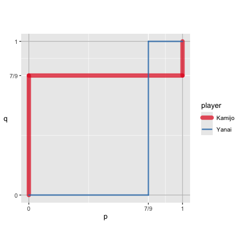
Example 3
An example of a normal-form game:
- Player:
- Strategy:
- Payoff:
You can define a game by specifying payoff functions as character vectors using normal_form():
game3 <- normal_form(
  players = c("A", "B"),
  payoffs1 = "-x^2 + (28 - y) * x",
  payoffs2 = "-y^2 + (28 - x) * y",
  par1_lim = c(0, 30),
  par2_lim = c(0, 30),
  pars = c("x", "y"))
Then, you can pass it to solve_nfg(), which displays the best response correspondences by default.
s_game3 <- solve_nfg(game3)
Example 4
An example of a normal-form game:
- Player:
- Strategy:
- Payoff:
You can define a normal-form game by specifying payoffs by R functions.
f_x <- function(x, y, a, b) {
-x^a + (b - y) * x
}
f_y <- function(x, y, s, t) {
-y^s + (t - x) * y
}
game4 <- normal_form(
players = c("A", "B"),
payoffs1 = f_x,
payoffs2 = f_y,
par1_lim = c(0, 30),
par2_lim = c(0, 30),
pars = c("x", "y"))Then, you can approximate a solution numerically by solve_nfg(). Note that you need to set the parameter values of the function that should be treated as constants by arguments cons1 and cons2, each of which accepts a named list. In addition, you can suppress the plot of best responses by plot = FALSE.
s_game4 <- solve_nfg(
game = game4,
cons1 = list(a = 2, b = 28),
cons2 = list(s = 2, t = 28),
plot = FALSE)
#> approximated NE: (9.3, 9.3)
#> The obtained NE might be only a part of the solutions.
#> Please examine br_plot (best response plot) carefully.You can increase the precision of approximation by precision, which takes a natural number (default is precision = 1).
s_game4b <- solve_nfg(
  game = game4,
  cons1 = list(a = 2, b = 28),
  cons2 = list(s = 2, t = 28),
  precision = 3)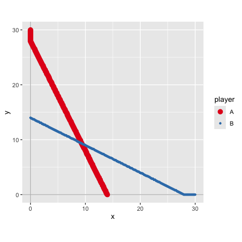
#> approximated NE: (9.333, 9.333)
#> The obtained NE might be only a part of the solutions.
#> Please examine br_plot (best response plot) carefully.
You can extract the best response plot with NE marked as follows.
s_game4b$br_plot_NE
Example 5
You can define payoffs by R functions and evaluate them at some discretized values by setting discretize = TRUE. The following is a Bertrand competition example:
func_price1 <- function(p, q) {
  if (p < q) {
    profit <- p
  } else if (p == q) {
    profit <- 0.5 * p
  } else {
    profit <- 0
  }
  profit
}

func_price2 <- function(p, q){
  if (p > q) {
    profit <- q
  } else if (p == q) {
    profit <- 0.5 * q
  } else {
    profit <- 0
  }
  profit
}

game5 <- normal_form(
  payoffs1 = func_price1,
  payoffs2 = func_price2,
  pars = c("p", "q"),
  par1_lim = c(0, 10),
  par2_lim = c(0, 10),
  discretize = TRUE)
Then, you can examine the specified part of the game.
s_game5 <- solve_nfg(game5, mark_br = FALSE)|
Player 2 |
|||||||
|---|---|---|---|---|---|---|---|
| strategy | 0 | 2 | 4 | 6 | 8 | 10 | |
| Player 1 | 0 | 0, 0 | 0, 0 | 0, 0 | 0, 0 | 0, 0 | 0, 0 |
| 2 | 0, 0 | 1, 1 | 2, 0 | 2, 0 | 2, 0 | 2, 0 | |
| 4 | 0, 0 | 0, 2 | 2, 2 | 4, 0 | 4, 0 | 4, 0 | |
| 6 | 0, 0 | 0, 2 | 0, 4 | 3, 3 | 6, 0 | 6, 0 | |
| 8 | 0, 0 | 0, 2 | 0, 4 | 0, 6 | 4, 4 | 8, 0 | |
| 10 | 0, 0 | 0, 2 | 0, 4 | 0, 6 | 0, 8 | 5, 5 | |
Example 6
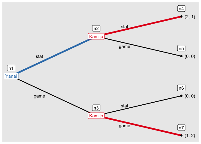
You can draw a tree of an extensive form game.
game6 <- extensive_form(
  players = list("Yanai",
                 rep("Kamijo", 2),
                 rep(NA, 4)),
  actions = list(c("stat", "game"),
                  c("stat", "game"), c("stat", "game")),
  payoffs = list(Yanai = c(2, 0, 0, 1),
                 Kamijo = c(1, 0, 0, 2)),
  direction = "right")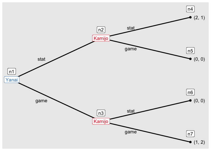
And you can find the solution of the game by solve_efg().
s_game6 <- solve_efg(game6)
#> backward induction: [(stat), (stat, game)]
Then, you can see the path played under a solution by show_path().
show_path(s_game6)